![]()

Learning objectives
In this lecture we cover the basics of NLP to build a sentiment classifier in scikit-learn. The learning goals are:
- Know the basics of string processing in python
- Preprocessing steps in NLP
- Count and TF-IDF encodings
- Naïve Bayes classifier
References
- Chapter 10: Representing and Mining Text in Data Science for Business by F. Provost and P. Fawcett
Homework
As homework read the references, work carefully through the notebook and solve the exercises.
Introduction to NLP
Natural language processing (NLP) concerns the part of Machine Learning about the analysis of digital, human written texts. The topic of NLP is as old as machine learning itself and dates back to Alan Turing himself. Since text is a widely used medium there are plenty of applications of machine learning:
- Text classification
- Question/answering systems
- Dialogue systems
- Named entity recognition
- Summarization
- Text generation
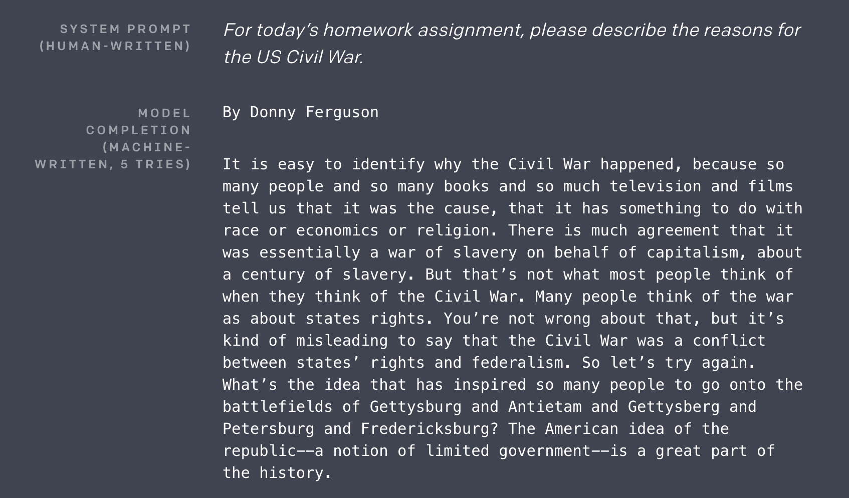
Especially in the past few years there has been exciting and rapid progress in the field. One example is the release of OpenAI's GPT-2, a language model able to not only create realistic text samples but also solve tasks of many NLP benchmarks without special training. See the figure below for an example output of GPT-2.
If you want to try your own examples you can do so at talktotransformer.com or read the original article on OpenAI's webpage.
Natural text is different to other data sources such as numerical tables or images. One way to look at text is to consider each word to be a feature. Since most languages have of the order of 100k words in their vocabulary plus many variations this leads to an enormous feature space. At the same time most words in the vocabulary do not appear in a small text. This leads to extreme sparsity. These properties call for a different approach to NLP than the methods we encountered and used for tabular data.
Notebook overview
The goal of this notebook is to classify movie reviews in terms of positive or negative feedback. This task is called sentiment analysis and is a common NLP application. As a company you might use a sentiment classifier to analyse customer feedback or detect toxic comments on your website.
Text data can be messy and require some clean up. The specific steps for the clean-up can depend on how the data was generated or where it was found. Text from the web might have some html artifacts that need cleaning or product reviews could include meta information on the review. Python offers powerful tools to manipulate strings. If cleaning requires complex rules one can also resort to regular expressions or regex for short.
Once the text is cleaned we have to encode it in a way that machine learning methods can handle. Directly using text representation as input is not possible. Most machine learning methods can only handle numerical data such as vectors and matrices. So we have to encode the input texts as vectors or matrices. These text representations are called vector encodings. Furthermore, we look at n-grams to keep some of the sequential structure of text.
Finally, we can train a model to classify the movie review texts. However, the Random Forest models we already know well do not work well for the high-dimensional data. We introduce a new methods that is common for text data called the Naïve Bayes classifier that utilises Bayes theorem.
import pandas as pd
import numpy as np
import pickle

import warnings
warnings.filterwarnings("ignore")

from dslectures.core import get_dataset

from tqdm import tqdm
tqdm.pandas(desc="progress")

import nltk
nltk.download('stopwords')
nltk.download('punkt')

from nltk import word_tokenize
from nltk.corpus import stopwords
from nltk.stem.snowball import SnowballStemmer

import seaborn as sns
import matplotlib.pyplot as plt

from sklearn.metrics.pairwise import cosine_similarity
from sklearn.feature_extraction.text import CountVectorizer, TfidfVectorizer
from sklearn.ensemble import RandomForestClassifier
from sklearn.naive_bayes import MultinomialNB
from sklearn.metrics import accuracy_score
First, we load the IMDB dataset as a dataframe. Note that this is not the original dataset from here, but a version that I pre-processed for the ease of use.
get_dataset('imdb.csv')
df_imdb = pd.read_csv('../data/imdb.csv')
df_imdb.head()
The dataset consists of a filename, text, sentiment and a train_label. The latter splits the data into a train and test set which is used as the official benchmark. We will follow that same split.
But first we want to make the sentiment column categorical:
df_imdb['sentiment'] = df_imdb['sentiment'].astype('category')
Now, let's have a look at a few text examples. For that purpose we wrote a helper function to print examples from the dataset:
def print_n_samples(df, n):
    """
    Helper function to print data samples from IMDB dataset.
    """
    for i in range(n):
        print('SAMPLE', i+1, '\n')
        df_sample = df.sample(1)
        print(df_sample['text'].values[0])
        print('\nSentiment:', df_sample['sentiment'].values[0],'\n')
        print("".join(100*['=']))
We can show a few examples:
print_n_samples(df_imdb, 2)
We can see that the reviews are medium sized texts with positive and negative labels.
Exercise 1
A few exploratory and processing tasks:
- Create a plot with showing the distribution of positive and negative comments in the train and test dataset.
- Study the distribution of the text lengths. You can perform string operations on a
pandas.DataFrameby accessing thestrobject of a column:df['YOUR_TEXT_COLUMN'].str.len().
In this section we have a look at the basics of string processing. Being able to filter/combine/manipulate strings is a crucial skill to do natural language processing.
Cleaning up text for NLP tasks usually involves the following steps.
- Normalization
- Tokenization
- Remove stop-words
- Remove non-alphabetical tokens
- Stemming
Some of the steps might not be necessary or you need to add steps depending on the text, task and method. For our task these steps are fine. We apply these steps on one text as an example and then build a function to apply it to all texts.
String processing in Python
Python offers powerful properties and functions to manipulate strings. The Python primer notebook offers an introduction to string processing with Python. Make sure to check it out. Once you are armed with this arsenal of string processing tools, we can preprocess the texts in the dataset to bring them to a cleaner form. Fortunately we don't need to implement everything from scratch. One of the richest Python libraries to process texts is the Natural Language Toolkit (NLTK) which offers some powerful functions we will use.
Exercise 2
Work through the string processing introduction in the Python primer notebook.
text = df_imdb.loc[0, 'text']
print(text)
text = text.lower()
print(text)
tokens = word_tokenize(text)
print(tokens)
stop_words = set(stopwords.words('english'))
print(stop_words)
We keep only the words that are not in the list of stop words.
tokens = [i for i in tokens if not i in stop_words]
print(tokens)
tokens = [i for i in tokens if i.isalpha()]
print(tokens)
Stemming
As a final step we want to trim the words to the stem. This helps drastically decrease the vocabulary size and maps similar/same words onto the same word. E.g. plural/singular words or different forms of verbs:
- pen, pens --> pen
- happy, happier --> happi
- go, goes --> go
There are several languages available in nltk since this is a language dependant process:
print(SnowballStemmer.languages)
Applied to the text sample this yields:
stemmer = SnowballStemmer("english")
tokens = [stemmer.stem(i) for i in tokens]
print(tokens)
def preprocessing(text, language='english', stemming=True):
    """
    preprocess a string and return processed tokens.
    args:
        text: text string
    return:
        tokens: list of processed and cleaned words
    """

    stop_words = set(stopwords.words(language))
    stemmer = SnowballStemmer(language)

    text = text.lower()
    tokens = word_tokenize(text)
    tokens = [i for i in tokens if not i in stop_words]
    tokens = [i for i in tokens if i.isalpha()]
    if stemming:
        tokens = [stemmer.stem(i) for i in tokens]

    return tokens
Finally, we can apply these steps to all texts. We use the apply function of pandas which applies a function to every entry in a DataFrame column. Since we registered tqdm we can use the progress_apply function which uses apply and adds a progress bar to it.
df_imdb['text_processed_stemmed'] = df_imdb['text'].progress_apply(preprocessing)
Now that we cleaned up and tokenized the text corpus we are now ready to encode the texts in vectors. In class we had a look at simple one-hot encodings that can be extended to count encodings and TF-IDF encodings.
Scikit-learn comes with functions to do both count and TF-IDF encodings on text. The interface is very similar to the classifier just the predict step is replace with transform:
count_vectorizer = CountVectorizer(your_settings)
count_vectorizer.fit(your_dataset)
vec = count_vectorizer.transform('your_text')
This creates a vectorizer that can transform texts to vectors. We can also limit the number of words take into account when building the vector. This limits the vector size and cuts off words that occur rarely. If you set max_features=10000 only the 10000 most occurring words are used to build the vector and all rare words are excluded. This means that the encoding vector then has a dimension of 10000. For now we take all words (max_features=None). Since we used our own tokenizer and preprocessing step we overwrite the standard steps in the vectorizer library with the vec_default_settings.
vec_default_settings = {'analyzer':'word', 'tokenizer':lambda x: x, 'preprocessor':lambda x: x, 'token_pattern':None,}
tfidf_vec = TfidfVectorizer(max_features=None, **vec_default_settings)
count_vec = CountVectorizer(max_features=None, **vec_default_settings)
Let's test both vectorizers on a small, dummy dataset with 4 documents:
corpus = [
    ['this','is','the','first','document','in','the','corpus'],
    ['this','document','is','the','second','document','in','the','corpus'],
    ['and','this','is','the','third','one','in','this','corpus'],
    ['is','this','the','first','document','in','this','corpus'],
]
Now we fit a count vectorizer to the data.
count_vec.fit(corpus)
Once the a vectorizer is fitted, we can investigate the vocabulary. It is a dictionary that points each word to the index in the vector it corresponds to. For example the word 'this' corresponds to the 10+1-nth (+1 because we start counting at zero) entry in the vector and the word 'and' corresponds to the the first entry.
len(count_vec.vocabulary_)
count_vec.vocabulary_
Now we can transform the corpus and get a list of vectors in the form of a matrix (each row corresponds to a document vector):
X = count_vec.transform(corpus)
print(X.toarray())
If we now do the same thing with the TF-IDF vectorizer we see that the output looks different:
tfidf_vec.fit(corpus)
X = tfidf_vec.transform(corpus)
print(X.toarray())
- The shape of the matrix is the same.
- Instead of integers (corresponding to counts) we have continous values.
- Elements that occur in multilple documents have lower scores than those appearing in fewer.
This should just illustrate how count and TF-IDF vectorizer work. Now let's apply this to our dataset and create encodigs with 100000 words:
n-grams
When we use a count or TF-IDF vectorizer we through away all sequential information in the texts. From the vector encodings above we could not reconstruct the original sentences. For this reason these encodings are called Bag-of-Words encodings (all words go in a bag and are shuffeled). However, sequential information can be important for the meaning of a sentence. As an example imagine the sentence:
text = 'The movie was good and not bad.'
It is important to know if the word 'not' is in front of 'good' or 'bad' for determining the sentiment of the sentence. We can preserve some of that information by using n-grams. Instead of just encoding single words we can also encode tuple, triplets etc. called n-grams. The n encodes how many words we bundle together.
The vectorizers can do this for us if we provide them a range of n's we want to include. In the following example we encode the text in 1- and 2-grams.
count_vec = CountVectorizer(max_features=None, ngram_range=(1,2), **vec_default_settings)
count_vec.fit(corpus)
We can see that this drastically increases the vocabulary.
len(count_vec.vocabulary_)
Now the vocabulary also contains word tuples next to the words:
count_vec.vocabulary_
The encodings look very similar but are larger due to the larger vocabulary:
X = count_vec.transform(corpus)
print(X.toarray())
max_features=100000
ngrams=(1,3)

count_vec = CountVectorizer(max_features=max_features, ngram_range=ngrams, **vec_default_settings)
In the example above we used the fit and transform function. We can avoid these two steps with the combined function fit_transform. First we need to split the dataset:
text_train = df_imdb.loc[df_imdb['train_label']=='train', 'text_processed_stemmed']
text_test = df_imdb.loc[df_imdb['train_label']=='test', 'text_processed_stemmed']
X_train = count_vec.fit_transform(text_train)
X_test = count_vec.transform(text_test)
This yields a vocabulary with 100000 entries:
len(count_vec.vocabulary_)
Looking at the shape of the returned matrix we see that it still has as many rows as the input but now has 100000 entries per row (the feature vector).
X_train.shape
Now that we featurised the text we can train a model on it. In this section we will use a Naïve Bayes classifier to determine whether a review is positive or negative. Firs we split the labels of the training and test set.
y_train = df_imdb.loc[df_imdb['train_label']=='train', 'sentiment']
y_test = df_imdb.loc[df_imdb['train_label']=='test', 'sentiment']
We can initialise a Naïve Bayes classifier the same way we initialised the Random Forest models. Also the fit/predict interface is the same.
nb_clf = MultinomialNB()
%%time
nb_clf.fit(X_train, y_train)
y_pred = nb_clf.predict(X_test)
We can calculate the prediction accuracy on the test set:
accuracy_score(y_test, y_pred)
rf_clf = RandomForestClassifier(n_jobs=-1)
%%time
rf_clf.fit(X_train, y_train)
y_pred = rf_clf.predict(X_test)
accuracy_score(y_test, y_pred)
We can see that we get similar performance while being ~1000x faster!
texts = ['This movie sucked!!',
         'This movie is awesome :)',
         'I did not like that movie at all.',
         'The movie was boring.']

enc = count_vec.transform(preprocessing(text) for text in texts)
print(nb_clf.predict(enc))