![]()

- Understand the main steps involved in exploratory data analysis
- Visualise geographical data with seaborn
- Slice, mask, and index
pandas.Seriesandpandas.DataFrameobjects - Merge
pandas.DataFrameobjects together on a common key - Apply the
DataFrame.groupby()operation to aggregate data across different groups of interest
This lesson draws heavily on the following textbook chapters:
- Chapter 2 of Hands-On Machine Learning with Scikit-Learn and TensorFlow by Aurèlien Geron
- Chapter 3 (pp. 146-170) of Python Data Science Handbook by Jake Vanderplas
You may also find the following blog post useful:
Homework
- Solve the exercises included in this notebook
- Work through lesson 2 and 4 from Kaggle Learn's introduction to pandas
If you get stuck on understanding a particular pandas technique, you might find their docs to be helpful.

In data science we apply the scientific method to data with the goal gain insights. This means that we state a hypothesis about the data, test it and refine it if necessary. In this framework, exploratory data analysis (EDA) is the step where we explore the data before actually building models. This helps us understand what information is actually contained in the data and what insights could be gained from it.
Formally, the goals of EDA are:
- Suggest hypotheses about the phenomena of interest
- Check if necessary data is available to test these hypotheses
- Make a selection of appropriate methods and models to achieve the goal
- Suggest what data should be gathered for further investigation
This exploratory phase lays out the path for the rest of a data science project and is therefore a crucial part of the process.
In this lesson we will analyse two datasets:
housing.csvhousing_addresses.csv
The first is the California housing dataset we saw in lesson 1, while the second provides information about the neighbourhoods associated with each house. This auxiliary data was generated using the reverse geocoding functionality from Google Maps, where the latitude and longitude coordinates for each house are converted into the closest, human-readable address.
The type of questions we will try to find answers to include:
- Which cities have the most houses?
- Which cities have the most expensive houses?
- What is the breakdown of the house prices by proximity to the ocean?
As in lesson 1, we will be making use of the pandas and seaborn libraries. It is often a good idea to import all your libraries in a single cell block near the top of your notebooks so that your collaborators can quickly see whether they need to install new libraries or not.
# reload modules before executing user code
%load_ext autoreload
# reload all modules every time before executing the Python code
%autoreload 2
# render plots in notebook
%matplotlib inline
# data wrangling
import pandas as pd
import numpy as np
from pathlib import Path
from dslectures.core import *

# data viz
import seaborn as sns
import matplotlib.pyplot as plt
import matplotlib.image as mpimg

# these commands define the color scheme
sns.set(color_codes=True)
sns.set_palette(sns.color_palette('muted'))
As usual, we can download our datasets using our helper function get_datasets:
get_dataset('housing.csv')
get_dataset('housing_addresses.csv')
We also make use of the pathlib library to handle our filepaths:
DATA = Path('../data/')
!ls {DATA}
housing_data = pd.read_csv(DATA/'housing.csv'); housing_data.head()
housing_addresses = pd.read_csv(DATA/'housing_addresses.csv'); housing_addresses.head()
Whenever we have a new dataset it is handy to begin by getting an idea of how large the DataFrame is. This can be done with either the len or DataFrame.shape methods:
# get number of rows
len(housing_data), len(housing_addresses)
# get tuples of (n_rows, n_columns)
housing_data.shape, housing_addresses.shape
Usually one finds that the column headers in the raw data are either ambiguous or appear in multiple DataFrame objects, in which case it is handy to give them the same name. Although it's obvious from the DataFrame.head() method what the column headers are for our housing and address data, in most cases one has tens or hundreds of columns and the fastest way to see their names is as follows:
housing_addresses.columns
Let's rename the route and locality-political columns to something more transparent:
housing_addresses.rename(columns={'route':'street_name', 'locality-political':'city'}, inplace=True)
# check that the renaming worked
housing_addresses.head()
DataFrame.rename() can manipulate an object in-place without returning a new object. In other words, when inplace=True is passed the data is renamed in place as data_frame.an_operation(inplace=True) so we don’t need the usual assignment LHS = RHS. By default, inplace=False so you have to set it explicitly if needed.Since we are dealing with data about California, we should check that the city column contains a reasonable number of unique entries. In pandas we can check this the DataFrame.nunique() method:
housing_addresses['city'].nunique()
In this lesson we will be focusing on how the house location affects its price, so let's make a scatterplot of the latitude and longitude values to see if we can identify any interesting patterns:
sns.scatterplot(x="longitude", y="latitude", data=housing_data);

Although the points look like the shape of California, we see that many are overlapping which obscures potentially interesting substructure. We can fix this by configuring the transparency of the points with the alpha argument:
sns.scatterplot(x="longitude", y="latitude", data=housing_data, alpha=0.1);

This is much better as we can now see distinct clusters of houses. To make this plot even more informative, let's colour the points according to the median house value; we will use the viridis colourmap (palette) as this has been carefully designed for data that has a sequential nature (i.e. low to high values):
fig = sns.scatterplot(
    x="longitude",
    y="latitude",
    data=housing_data,
    alpha=0.1,
    hue="median_house_value",
    palette="viridis",
    size=housing_data["population"] / 100
)

# place legend outside of figure
fig.legend(loc="center left", bbox_to_anchor=(1.01, 0.6), ncol=1);

Finally, to make our visualisation a little more intuitive, we can also overlay the scatter plot on an actual map of California:
fig = sns.scatterplot(
    x="longitude",
    y="latitude",
    data=housing_data,
    alpha=0.1,
    hue="median_house_value",
    palette="viridis",
    size=housing_data["population"] / 100
)

# place legend outside of figure
fig.legend(loc="center left", bbox_to_anchor=(1.01, 0.6), ncol=1);

# ref - www.kaggle.com/camnugent/geospatial-feature-engineering-and-visualization/
california_img=mpimg.imread('images/california.png')
plt.imshow(california_img, extent=[-124.55, -113.80, 32.45, 42.05], alpha=0.5);

Although the housing_data and housing_addresses DataFrames contain interesting information, it would be nice if there was a way to join the two tables.
More generally, one of the most common operations in pandas (or data science for that matter) is the combination of data contained in various objects. In particular, merge or join operations combine datasets by linking rows using one of more keys. These operations are central to relational databases (e.g. SQL-based). The pandas.merge() function in pandas is the main entry point for using these algorithms on your data.
Let's use this idea to combine the housing_data and housing_addresses pandas.DataFrame objects via their common latitude and longitude coordinates. First we need to combine the latitude and longitude columns of housing_data into the same lat,lon format as our housing_addresses pandas.DataFrame. To do so, we will use the Series.astype() function to convert the numerical column values to strings, then use string concatenation to create a new latitude_longitude column with the desired format:
# create new column
housing_data['latitude_longitude'] = housing_data['latitude'].astype(str) + ',' + housing_data['longitude'].astype(str)
# check the column was created
housing_data.head()
Now that we have latitude_longitude present in both pandas.DataFrame objects we can merge the two tables together in pandas as follows:
# create a new DataFrame from the merge
housing_merged = pd.merge(
    housing_data, housing_addresses, how="left", on="latitude_longitude"
)
# check merge worked
housing_merged.head()
Boom! We now have a single pandas.DataFrame that links information for house prices and attributes and their addresses.
latitude_longitude found in the left table housing_data. In general the 'how' argument of pandas.merge() allows four different join types:
'left': Use all key combinations found in the left table'right': Use all key combinations found in the right table'inner': Use only the key combinations observed in both tables'outer': Use all key combinations observed in both tables together
A visual example of these different merges in action is shown in the figure below.
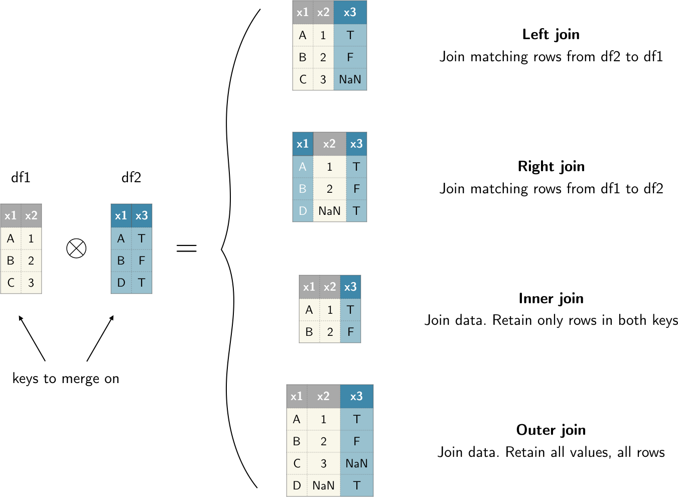
Figure: Graphical representation of the different types of merges between two DataFrames df1 and df2 that are possible in pandas.
pandas.DataFrame you can expect a larger table to appear after you do a left join. To avoid this behaviour, you can run DataFrame.drop_duplicates() before doing the merge.It is not uncommon for a dataset to have tens or hundreds of columns, and in practice we may only want to focus our attention on a smaller subset. One way to remove unwanted columns is via the DataFrame.drop() method. Since we have duplicate information about the latitude and longitude coordinate, we may as well drop the latitude_longitude column from our merged pandas.DataFrame:
# inplace=True manipulates an object without returning a new object
housing_merged.drop(['latitude_longitude'], axis=1, inplace=True); housing_merged.head()
pandas.DataFrame and pandas.Series objects. This parameter is used to specify along which dimension we want to apply a given transformation - see the figure below for a graphical representation.
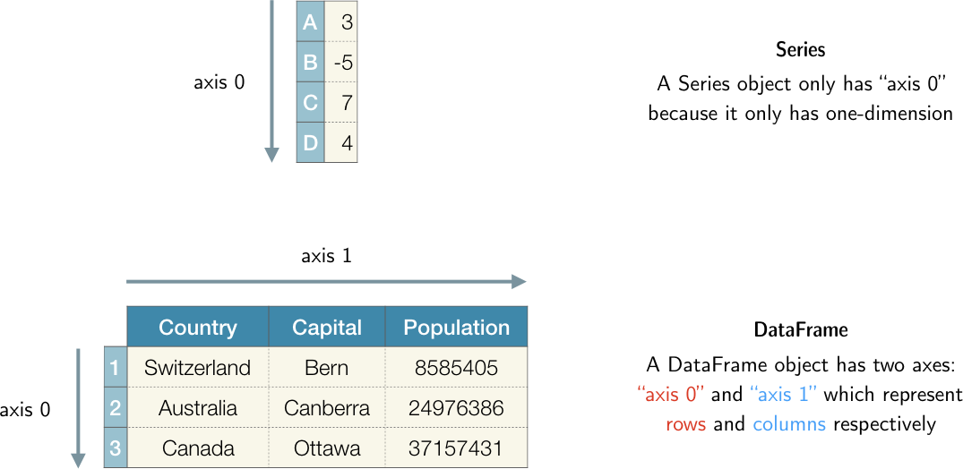
Figure: Visualisation of the axis parameter in pandas.
At this point, we have a unfified table with housing data and their addresses. This is usually a good point to save the intermediate results to disk so that we can reload them without having to run all preprocessing steps. To do so in pandas, we can make use of the DataFrame.to_csv() function:
# use index=False to avoid adding an extra column for the index
housing_merged.to_csv(path_or_buf=DATA/'housing_merged.csv', index=False)
Now that we have a tidy pandas.DataFrame let's apply some of the most common pandas methods to make queries on the data.
A pandas.Series object provides array-style item selection that allows one to perform slicing, masking, and fancy indexing. For example, we can study the housing_median_age colum from a variety of angles:
# define a new Series object
age = housing_merged['housing_median_age']
age
# get first entry
age[0]
# slicing by index
age[2:5]
# slice and just get values
age[2:5].values
age.describe()
# masking (filtering)
age[(age > 10.0) & (age < 20.0)]
# fancy indexing
age[[0, 4]]
Since a pandas.DataFrame acts like a two-dimensional array, pandas provides special indexing operators called DataFrame.iloc[] and DataFrame.loc[] to slice and dice our data. As an example, let's select a single row and multiple columns by label:
housing_merged.loc[2, ['city', 'population']]
We can perform similar selections with integers using DataFrame.iloc[]:
housing_merged.iloc[2, [3, 11]]
Masks or filters are especially common to use, e.g. let's select the subset of expensive houses:
housing_merged.loc[housing_merged['median_house_value'] > 450000]
We can also use Python's string methods to filter for things like
housing_merged.loc[housing_merged['ocean_proximity'].str.contains('O')]
pandas.Series and pandas.DataFrame objects is the fact that they contain an index that lets us slice and modify the data. This Index object can be accessed via Series.index or DataFrame.index and is typically an array of integers that denote the location of each row.For example, our age object has an index for each row or house in the dataset:
age.index
We can also sort the values according to the index, which in our example amounts to reversing the order:
age.sort_index(ascending=False)
Finally, there are times when you want to reset the index of the pandas.Series or pandas.DataFrame objects; this can be achieved as follows:
age.reset_index()
Note this creates a new index column and resets the order of the pandas.Series object in ascending order.
Whenever you need to quickly find the frequencies associated with categorical data, the DataFrame.value_counts() and Series.nlargest() functions come in handy. For example, if we want to see which city has the most houses, we can run the following:
housing_merged['city'].value_counts().nlargest(10)
This seems to make sense, since Los Angeles, San Diego, and San Francisco have some of the largest populations. We can check whether this is indeed the case by aggregating the data to calculate the total population value across the group of cities. pandas provides a flexibly DataFrame.groupby() interface that enables us to slice, dice, and summarise datasets in a natural way. In particular, pandas allows one to:
- Split a pandas object into pieces using one or more keys
- Calculate group summary statistics, like count, mean, standard deviation, or a user-defined function
- Apply within-group transformations or other manipulations, like normalisation, rank, or subset selection
- Compute pivot tables and cross-tabulations.
Let's combine these ideas to answer our question, followed by an explanation of how the GroupBy mechanics really work:
housing_merged.groupby('city').agg({'population':'sum'})
This seems to work - we now have the average number of people residing in a block of houses, but the result seems to be sorted alphabetically. To get the cities with the largest populations, we can use the Series.sort_values() method as follows:
housing_merged.groupby("city").agg({"population": "sum"}).sort_values(
    by="population", ascending=False
)
That's much better! We can store the result as a new pandas.DataFrame and plot the distribution:
# use outer parentheses () to add line breaks
top10_largest_cities = (
    # group by key=city
    housing_merged.groupby("city")
    # calculate total population
    .agg({"population": "sum"})
    # select 10 largest
    .nlargest(10, columns="population")
    # reset index so city becomes column
    .reset_index()
)
top10_largest_cities.head()
sns.barplot(x='population', y='city', data=top10_largest_cities, color='b');

The group operation above can be best understood by the H. Wickam's split-apply-combine strategy, where you break up a big problem into manageable pieces, operate on each piece independently and then put all the pieces back together.
Split:
In the first stage of the process, data contained in a pandas.Series or pandas.DataFrame object is split into groups based on one or more specified keys. The splitting is performed on a particular axis of the object (see the notebook from lesson 2). For example, a pandas.DataFrame can be grouped on its rows (axis=0) or its columns (axis=1).
Apply: Once the split done, a function is applied to each group, producing a new value.
Combine: Finally, the results of all those function applications are combined into a result object. The form of the resulting object will usualy depend on the what's being done to the data.
See the figure below for an example of a simple group aggregation.
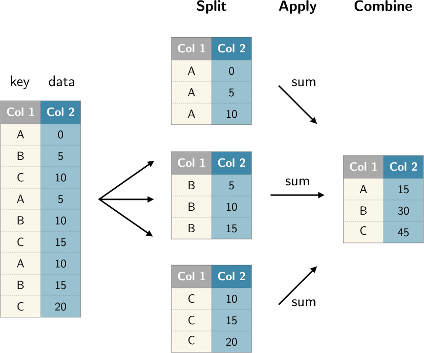
Figure: Illustraion of a group aggregation.
In general, the grouping key can take many forms and the key do not have to be all of the same type. Frequently, the grouping information is found in the same pandas.DataFrame as the data you want to work on, so the key is usually a column name. For example let's create a simple pandas.DataFrame as follows:
df_foo = pd.DataFrame(
    {
        "key1": ["a", "a", "b", "b", "a"],
        "key2": ["one", "two", "one", "two", "one"],
        "data1": np.random.randn(5),
        "data2": np.random.randn(5),
    }
)
df_foo
We can then use the column names as the group keys (similar to what we did above with the beers):
grouped = df_foo.groupby('key1'); grouped
This grouped variable is now a GroupBy object. It has not actually calculated anything yet except for some intermediate data about the group key df_foo['key1']. The main idea is that this object has all of the information needed to then apply some operation to each of the groups. For example, we can get the mean per group as follows:
df_grouped = grouped.mean(); df_grouped
Exercise #5
- Use the above
DataFrame.groupby()techniques to find the top 10 cities which have the most expensive houses on average. Look up some of the names on the web - do the results make sense? - Use the
DataFrame.loc[]method to filter out the houses with the capped values of over $500,000. Repeat the same step as above.