![]()

- Understand the main steps involved in preparing data for machine learning algorithms
- Create Python functions to automate steps of the data cleaning process
- Gain an introduction to matplotlib's object-oriented interface to combine plots on the same figure
This lesson draws heavily on the following textbook chapter:
- Chapter 2 of Hands-On Machine Learning with Scikit-Learn and TensorFlow by Aurèlien Geron
You may also find the following blog posts useful:
- Machine Learning with Kaggle: Feature Engineering
- Sections 2 and 3 of Intermediate Machine Learning on Kaggle Learn
- Effectively Using Matplotlib by C. Moffitt

When you receive a new dataset at the beginning of a project, the first task usually involves some form of data cleaning.
To solve the task at hand, you might need data from multiple sources which you need to combine into one unified table. However, this is usually a tricky task; the different data sources might have different naming conventions, some of them might be human-generated, while others are automatic system reports. A list of things you usually have to go through are the following:
- Merge multiple sources into one table
- Remove duplicate entries
- Clean corrupted entries
- Handle missing data
In lesson 2, we examined how to merge the table of housing data with their addresses; in this lesson we will focus on the remainign three steps.
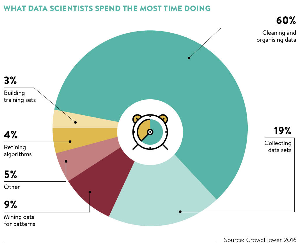
Although building algorithms that are able to classify data or estimate outcomes is arguably the most interesting part of data science, data cleaning is the one that takes up most of the time. According to a study by CrowdFlower, data scientists spend about 60-80% of their time preparing datasets for machine learning algorithms.
In this lesson we will analyse the unified table of housing data and their addresses that we created in lesson 2:
housing_merged.csv
As in previous lessons, we will be making use of the pandas and seaborn libraries.
# reload modules before executing user code
%load_ext autoreload
# reload all modules every time before executing the Python code
%autoreload 2
# render plots in notebook
%matplotlib inline
# data wrangling
import pandas as pd
import numpy as np
from pathlib import Path
from dslectures.core import *

# data viz
import seaborn as sns
import matplotlib.pyplot as plt
import matplotlib.image as mpimg

# these commands define the color scheme
sns.set(color_codes=True)
sns.set_palette(sns.color_palette('muted'))
As usual, we can download our datasets using our helper function get_datasets:
get_dataset('housing_merged.csv')
We also make use of the pathlib library to handle our filepaths:
DATA = Path('../data/')
!ls {DATA}
housing_data = pd.read_csv(DATA/'housing_merged.csv'); housing_data.head()
Before we prepare the data for training machine learning models, it is useful to experiment with creating new features (i.e. columns) that may provide more information than the raw data alone. For example the column total_rooms refers to the total number of rooms in a housing district, and thus it is more useful to know the number of rooms per household. In pandas, we can create this new column as follows:
housing_data['rooms_per_household'] = housing_data['total_rooms'] / housing_data['households']
# check we have added the column
housing_data.head(1)
Exercise #1
- Create a new feature called
bedrooms_per_householdfrom thetotal_bedroomsandhouseholdsfeatures - Create a new feature called
bedrooms_per_roomfrom thetotal_bedroomsandtotal_roomsfeatures - Create a new feature called
population_per_householdfrom thepopulationandhouseholdsfeatures - Recalculate the correlation matrix from lesson 1 - what can you conclude about the correlation of the new features with the median house value?
Recall from lesson 1 that the quantity we wish to predict (median house value) has a cap around $500,000:
# use plt.subplots() to create multiple plots
fig, (ax0, ax1) = plt.subplots(nrows=1, ncols=2, figsize=(7, 4))
# put one plot on axis ax0
sns.distplot(housing_data["median_house_value"], kde=False, ax=ax0)
# put second plot on axis ax1
sns.scatterplot("median_income", "median_house_value", data=housing_data, ax=ax1)
# tight_layout() fixes spacing between plots
fig.tight_layout()

The presence of this cap is potentially problematic since our machine learning algorithms may learn that the housing prices never go beyond that limit. Let's assume that we want to predict housing prices above $500,000, in which case we should remove these districts from the dataset.
Exercise #2
- Store the number of rows in
housing_datain a variable calledn_rows_raw - Use the
DataFrame.loc[]method to remove all rows wheremedian_house_valueis greater than or equal to $500,000 - Calculate the fraction of data that has been removed by this filter.
- Create new histogram and scatter plots to make sure you have removed the capped values correctly.
If we inspect the data types associated with our housing pandas.DataFrame
housing_data.dtypes
we see that in addition to numerical features, we have features of object data type, which pandas denotes with the string O:
housing_data['ocean_proximity'].dtype
# compare against numerical column
housing_data['median_house_value'].dtype
pandas has a handy set of functions to test the data type of each column. For example, to check whether a column is of object or numeric type we can import the following functions
from pandas.api.types import is_object_dtype, is_numeric_dtype
and then test them against some columns:
is_object_dtype(housing_data['ocean_proximity'])
is_numeric_dtype(housing_data['ocean_proximity'])
is_numeric_dtype(housing_data['median_house_value'])
In this case, we know these columns are strings and some step is needed to convert them to numerical form because most machine learning algorithms are best suited for doing computations on arrays of numbers, not strings.
pandas has a special Categorical type for holding data that uses the integer-based categorical representation or encoding. For example housing_data['ocean_proximity'] is a pandas.Series of Python string objects ['NEAR BAY', '<1H OCEAN', 'INLAND', 'NEAR OCEAN', 'ISLAND']. We can convert a pandas.DataFrame column to categorical as follows:
housing_data['ocean_proximity'] = housing_data['ocean_proximity'].astype('category')
The resulting Categorical object has categories and codes attributes that can be accessed as follows:
housing_data['ocean_proximity'].cat.categories
housing_data['ocean_proximity'].cat.codes
Categorical features as text and treat them internally as numerical.Sometimes we may want to reorder by hand the categorical variables. For example, with our ocean_proximity feature, it makes more sense to order the categories by distance to the ocean:
housing_data["ocean_proximity"].cat.set_categories(
    ["INLAND", "<1H OCEAN", "NEAR BAY", "NEAR OCEAN", "ISLAND"], ordered=True, inplace=True
)
Exercise #3
- Create a function called
convert_strings_to_categoriesthat takes apandas.DataFrameas an argument and converts all columns ofobjecttype intoCategorical. Note that the operation can be done in-place and thus your function should not return any objects. You may find the commandsDataFrame.columnsandis_numeric_dtypeare useful. - Check that the transformed
housing_datahas the expected data types.
In general, machine learning algorithms will fail to work with missing data, and in general you have three options to handle them:
- Get rid of the corresponding rows
- Get rid of the whole feature or column
- Replace the missing values with some value like zero or the mean, median of the column.
A quick way to check if there's any missing data is to run the pandas DataFrame.info() method:
housing_data.info()
Since housing_data has 20,640 rows we see that the following columns are missing values:
total_bedroomsstreet_numberstreet_namecitypostal_codebedrooms_per_householdbedrooms_per_room
An alternative way to verify this is to apply the DataFrame.isnull() method and calculate the sum of missing values in housing_data:
housing_data.isnull().sum()
Exercise #4
It is often more informative to know the fraction or percentage of missing values in a pandas.DataFrame.
- Calculate the fraction of missing values in
housing_dataand sort them in descending order. - Use seaborn to create a bar plot that shows the fraction of missing data that you calculated above.
Let's look at our first option to handle missing data: getting rid of rows. One candidate for this is the city column since dropping the 188 rows amounts to less than 1% of the total dataset. To achieve this we can use the DataFrame.dropna() method as follows:
housing_data.dropna(subset=['city'], inplace=True)
# check city has no missing values
housing_data['city'].isnull().sum()
We still have missing values for the categorical features street_number and street_name. For such data one simple approach is to replace the missing values with the most frequent entry. However, for these specific attributes it does not make much sense to replace e.g. the missing street names with the most common ones in some other city.
To that end, we will drop the street_number and street_name columns.
For the numerical columns, let's replace the missing values by the median.
For example, with total_bedrooms this might look like the following:
# calculate median total number of bedrooms
total_bedrooms_median = housing_data['total_bedrooms'].median()
# use inplace=True to make replacement in place
housing_data['total_bedrooms'].fillna(total_bedrooms_median, inplace=True)
# check replacement worked
housing_data['total_bedrooms'].isnull().sum()
Although doing this replacement manually for each numerical column is feasible for this small dataset, it would be much better to have a function that automates this process.
Exercise #7
- Create a function called
fill_missing_values_with_medianthat takes apandas.DataFrameas an argument and replaces missing values in each column with the median. Note that the operation can be don in-place, so your function should not return any objects. You may find the commandis_numeric_dtypeto be useful. - Check that missing values are filled in the transformed
pandas.DataFrame.
We've now reached the stage where we have a cleaned pandas.DataFrame and the final step is to convert our categorical columns to numerical form. For example, we can numericalise the city column by replacing the categories with their corresponding codes:
# add +1 so codes start from 1
housing_data['city'] = housing_data['city'].cat.codes + 1
# check output
housing_data.head(1)
One potential problem with the above representation is that machine learning algorithms will treat two cities that are numerically close to each other as being similar. Thus an alternative approach is to apply a technique known as one-hot encoding, where we create a binary feature per category. In pandas we can do this by simply running pandas.get_dummies():
housing_data = pd.get_dummies(housing_data)
housing_data.head()
Note that the above has converted our ocean_proximity column into one new column per category!
city or post_code columns, even though they are strictly categorical.# sanity check
housing_data.info()
housing_data.to_csv(DATA/'housing_processed.csv', index=False)