![]()

Learning Objectives
Overfitting is a phenomena that can always occur when a model is fitted to data. Therefore, it is important to understand what it entails and how it can be avoided. In this notebook we will address these three questions related to overfitting:
- What is overfitting?
- How can we measure overfitting?
- How can overfitting be avoided?
References
- Chapter 5: Overfitting and its avoidance of Data Science for Business by F. Provost and P. Fawcett
Homework
- Work through part 2 of the notebook concerning the housing dataset.
- Solve exercises in the notebook. In particular, tune a random forest for the churn dataset in part 3.
What is overfitting?
Already John von Neumann, one of the founding fathers of computing, knew that fitting complex models to data is a tricky business:
With four parameters I can fit an elephant, and with five I can make him wiggle his trunk.
- John von Neumann

Figure reference:Irrelevant image.
When we fit a model to data we always have to be careful not to overfit. If we overfit the model this means that the model learned specific aspects of the training data and does not generalise to new, unseen data. Instead of learning useful relations between the input feature and the target the model has memorised the training samples. If this happens the model we perform very poorly on new data and therefore we want to make sure this does not happen.
Fortunately, there are tools that can help detect and avoid overfitting. One tool we already used: splitting the data into two sets. Measuring the performance difference between the training and validation set already helps identifying when we are overfitting. In this lecture we will see an even more systematic way of splitting the data namely cross-validation.
# reload modules before executing user code
%load_ext autoreload
# reload all modules every time before executing Python code
%autoreload 2
# render plots in notebook
%matplotlib inline
import numpy as np
import seaborn as sns
import pandas as pd
import matplotlib.pyplot as plt
from pathlib import Path
from tqdm import tqdm
import time

from sklearn.model_selection import train_test_split, cross_validate
from sklearn.ensemble import RandomForestRegressor, RandomForestClassifier

from dslectures.core import rmse, make_polynomial_data, PolynomialRegressor, get_dataset
from dslectures.structured import proc_df

np.warnings.filterwarnings('ignore')
Part 0: tqdm
Before starting with overfitting we introduce the tqdm library. In this notebook we will make extensive use of for-loops and tqdm is a very handy addition to them. With just one expression you can add a progress bar to your for loop. Let say you have a for-loop that does some computation:
for i in range(1000):
    #do something
    a = i**2
    time.sleep(0.01)
for i in tqdm(range(1000)):
    #do something
    a = i**2
    time.sleep(0.01)
sum_i = 0
for i in tqdm([1,2,3,4,5]):
    sum_i += i
    time.sleep(1)
print('sum:', sum_i)
Part 1: Overfitting Polynomials
Polynomials
To study the nature of overfitting we start looking at a the toy example of a polynomials. Later we will see our findings are not specific to polynomials and can be extended to other supervised machine learning methods such as linear regressors, tree classifiers or random forests.
A polynomial of degree $n$ has the form: $$f(x) = w_0 + w_1\cdot x + w_2\cdot x^2 +\ldots+w_n\cdot x^n$$
Generate data
In this block we generate a random polynomial of degree 3 With the helper function get_polynomial_data. The polynomial has the form:
$$f(x) = 10 \cdot x^3 -5 \cdot x $$
If you are interested in creating or fitting polynomial data check out the functions numpy.polyval and numpy.polyfit. In this lesson we will use wrapper functions around them. The function get_polynomial_data(w, n_samples=100) evaluates the polymial defined by w on n_samples random points and adds some noise to it.
weights = np.array([10, 0, -5, 0])
X, y = make_polynomial_data(weights, n_samples=100)
We can plot the polynomial data in a scatter plot:
def scatter_plot_polynomial(X, y, label='', title='Polynomial data'):
    plt.title(title)
    plt.scatter(X, y, label=label)
    plt.xlabel('x')
    plt.ylabel('y')
    plt.grid(True)
    plt.legend(loc='best')
scatter_plot_polynomial(X, y, label='data')
plt.show()

X_train, X_valid, y_train, y_valid = train_test_split(X, y, test_size=0.2,)
scatter_plot_polynomial(X_train, y_train, label='training set')
scatter_plot_polynomial(X_valid, y_valid, label='validation set')

Now lets fit a polynomial to the generated data. We can use PolyFit class to fit a polynomial to the data. We can pass the the degree as an argument and then use the same functions fit, predict and evaluate functions known from scikit-learn.
pr = PolynomialRegressor(degree=3)
pr.fit(X_train, y_train)
Now we want to see how that polynomial looks like on a range from [-1, 1]:
X_lin = np.linspace(-1, 1, 1000)
y_fit = pr.predict(X_lin)
scatter_plot_polynomial(X_train, y_train, label='training set')
scatter_plot_polynomial(X_valid, y_valid, label='validation set')
plt.plot(X_lin, y_fit, label='fit', c='black')
plt.show()

We can investigate the shape of the fitted curve for different values of degree:
for degree in [0, 1, 2, 3, 5, 10, 50]:
    pr = PolynomialRegressor(degree=degree)
    pr.fit(X_train, y_train)
    y_fit = pr.predict(X_lin)

    title = f'Polynomial fit degree={degree}'
    scatter_plot_polynomial(X_train, y_train, label='polynomial data', title=title)
    scatter_plot_polynomial(X_valid, y_valid, label='validation set', title=title)
    plt.plot(X_lin, y_fit, label='fit', c='black')

    plt.ylim([-6, 6])
    plt.show()


By just looking at the curves we can observe 3 regimes:
Underfitting (degree<3): The model is not able to fit the complexity data properly. The fit is bad for both the training and the validation set.
Fit is just right (degree=3): The model is able to caputre the underlying data distribution. The fit is good for both the training and the validation set.
Overfitting (degree>3: The model starts fitting the noise in the dataset. While the fit for the training data gets even better the fit for the validation set gets worse.
rmse_train = []
rmse_valid = []
degrees = list(range(0, 30))

for degree in tqdm(degrees):
    pr = PolynomialRegressor(degree=int(degree))
    pr.fit(X_train, y_train)
    rmse_train.append(pr.evaluate(X_train, y_train))
    rmse_valid.append(pr.evaluate(X_valid, y_valid))
def plot_fitting_graph(x, metric_train, metric_valid, metric_name='metric', xlabel='x', yscale='linear'):
    plt.plot(x, metric_train, label='train')
    plt.plot(x, metric_valid, label='valid')
    plt.yscale(yscale)
    plt.title('Fitting graph')
    plt.ylabel(metric_name)
    plt.xlabel(xlabel)
    plt.legend(loc='best')
    plt.grid(True)
plot_fitting_graph(degrees, rmse_train, rmse_valid, metric_name='RMSE', xlabel='degree')

We can make a few observations:
- The training error always decreases when adding more degrees.
- There is a region between 3-15 where the validation error is stable and low.
Ideally, we would choose the the model parameters such that we have the best model performance. However, we want to make sure that we really have the best validation performance. When we do train_test_split we randomly split the data into to parts. What could happen is that we got lucky and split the data such that it favours the validation error. This is especially dangerous if we are dealing with small datasets. One way to check if that's the case is to run the experiment several times for different, random splits. However, there is an even more systematic way of doing this: cross-validation.
Cross-validation
The idea behind cross validation is to split the data into k equally sized parts, called folds. Each fold gets to be the validation set once while the other folds play the training set part. That means we run k experiments and aggregate the training and validation metrics by averaging them. This is a more robust approach to monitoring overfitting and thanks to scikit-learn we only have to adjust one line by adding the cross_validate function!
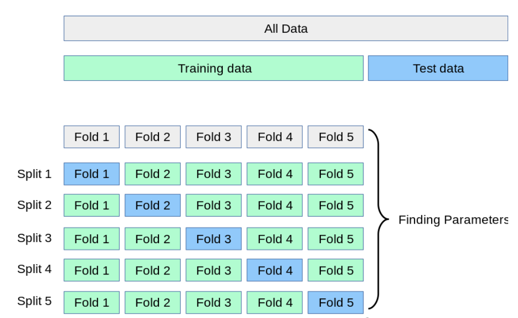
Figure reference: https://scikit-learn.org/stable/modules/cross_validation.html
Cross-valida takes care of all the steps, we just have to pass an initialized model, the full dataset and the number of folds with the keyword cv. Furthermore, we need to specify the metric to be evaluated and also that we want it to return the scores on the training sets.
rmse_train = []
rmse_valid = []
degrees = list(range(0, 16))
for degree in tqdm(degrees):
    pr = PolynomialRegressor(degree=degree)
    results = cross_validate(pr, X, y,
                             cv=5,
                             return_train_score=True,
                             scoring='neg_root_mean_squared_error')

    # we average the scores and append them to the list
    rmse_train.append(-np.mean(results['train_score']))
    rmse_valid.append(-np.mean(results['test_score']))
plot_fitting_graph(degrees, rmse_train, rmse_valid, metric_name='RMSE', xlabel='degree', yscale='log')

We can use np.argmin to find the element with the minimum validation error. The function returns the index in the array with the minimum value.
np.argmin(rmse_valid)
Since we start counting from 0 in programming this means we are looking for the fourth element in the degrees list:
degrees
degrees[np.argmin(rmse_valid)]
In these experiments we made some key observations:
- We can fit polynomials (hurray)
- There are three regimes when fitting polynomials: underfitting, good fit and overfitting
- These regimes depend on the degree of the polynomials we are fitting.
- Increasing the degree of the polynomials always decreases the training error.
- The validation error decreases in the from the underfitting to good fit regime and then increases in the overfitting region.
These observations are not special about polynomials - they hold for fitting machine learning models in general. Let's translate these observations to general machine learning models:
The challenge in fitting models in machine learning is to find the good fit. A model that is too simple will not be able to capture the complexity of the data and lead to underfitting. A model that is too complex has the capacity to "memorize" aspects of the data and cause overfitting. If we are overfitting our model will not predict well unseen data - we say it does not generalise. The goal is to find a model that has just the right complexity to fit the data. The fitting graph is a tool to identify the sweetspot of model complexity.
Complexity
The model complexity comes in different form and shapes. In our polynomial example the complexity is controlled by the degree parameter. For a Random Forest the complexity is given by several parameters such as tree_depth of and n_estimators.
Classification
We can also create fitting graphs for classification tasks. Instead of looking at RMSE we can look at the accuracy. The difference is that the graph will look inverted in the y-axis; instead of looking for the lowest validation error we will look for the highest validation accuracy.
More data
There is another way to reduce overfitting: get more data! In the following exercise you explore how more data influences the fitting graph.
Exercise #1
Use the get_polynomial_data and generate 100_000 samples. Create another fitting graph with cross-validation and compare it to the one with 100 samples.
In the following section we will investigate overfitting in Random Forests.
Train/validation/test set
Before we move to RandomForests we want to clarify some ambiguity about the terms train, validation and test set. So far we have concentrated on the train and validation set: We train a model on the train set and we evaluate the metrics on the validation set. However, sometimes we also come across the term test set. For example the function we used to split the dataset in to sets: train_test_split.
In machine learning each of these sets has a distinct function:
- The train set is used to train a model.
- With the validation set the model is evaluated. With this information we tune the parameters.
- We only evaluate the final, tuned model on the test set. We do not use it to tune the model parameters.
The reason we make the distinction between validation and test set is that by tuning the parameters on the validation performance we might start to overfit the validation data. The test set gives a final sanity check that we actually have a performant model.
In cross-validation the concept of train and validation is melted and all training data is also validation data at some point.
Part 2: Housing dataset
In this section we want to use cross-validation to sytematically tune the parameters of the Random Forest without overfitting. We do it in a linear fashion and tune one parameter after another. This does not guarantee that we find the best global parameters, but runs much faster than a global grid search. We will tune the following parameters:
- n_estimators
- max_depth
- min_samples_leaf
- max_features
First we load the processed housing data:
get_dataset('housing_processed.csv')
DATA = Path('../data/')
!ls {DATA}
housing_data = pd.read_csv(DATA/'housing_processed.csv')
housing_data.head()
X = housing_data.drop('median_house_value', axis=1)
y = housing_data['median_house_value']
rf = RandomForestRegressor(n_jobs=-1)
results = cross_validate(rf, X, y,
                         cv=5,
                         return_train_score=True,
                         scoring='neg_root_mean_squared_error')
print('Train score: %.1f' % -np.mean(results['train_score']))
print('Validation score: %.1f' % -np.mean(results['test_score']))
Now we tune one parameter after another and always choose the best one of the round based on the fitting curve.
rmse_train = []
rmse_valid = []

n_estimators = [25, 50, 100, 200]
for n in tqdm(n_estimators):
    rf = RandomForestRegressor(n_estimators=n, n_jobs=-1)
    results = cross_validate(rf, X, y,
                             cv=5,
                             return_train_score=True,
                             scoring='neg_root_mean_squared_error')

    # we average the scores and append them to the list
    rmse_train.append(-np.mean(results['train_score']))
    rmse_valid.append(-np.mean(results['test_score']))
plot_fitting_graph(n_estimators, rmse_train, rmse_valid, metric_name='RMSE', xlabel='n_estimators')

We can zoom in a little bit further to get a better picture of how the validation error behaves:
We see that adding more estimaters further decreases the validation error. We do not overfit by adding more estimators. However, it takes longer to train and evaluate the model as we add more estimators. This is usually not a major concern when experimenting with models but it can be a major constraint when putting it in production. See this example from Netflix.
We choose n_estimators=100 for the sake of speed but we keep in mind that we could probably further improve the model by adding more estimators. We continue tuning the other parameters:
rmse_train = []
rmse_valid = []

max_depths = [1, 2, 4, 8, 16, 32, 64]
for d in tqdm(max_depths):
    rf = RandomForestRegressor(n_estimators=100, max_depth=d, n_jobs=-1)
    results = cross_validate(rf, X, y,
                             cv=5,
                             return_train_score=True,
                             scoring='neg_root_mean_squared_error')

    # we average the scores and append them to the list
    rmse_train.append(-np.mean(results['train_score']))
    rmse_valid.append(-np.mean(results['test_score']))
plot_fitting_graph(max_depths, rmse_train, rmse_valid, metric_name='RMSE', xlabel='max_depths')

max_depths[np.argmin(rmse_valid)]
rmse_train = []
rmse_valid = []

min_samples_leaf = [1, 3, 5, 10, 25]
for s in tqdm(min_samples_leaf):
    rf = RandomForestRegressor(n_estimators=100, max_depth=16, min_samples_leaf=s, n_jobs=-1)
    results = cross_validate(rf, X, y,
                             cv=5,
                             return_train_score=True,
                             scoring='neg_root_mean_squared_error')

    # we average the scores and append them to the list
    rmse_train.append(-np.mean(results['train_score']))
    rmse_valid.append(-np.mean(results['test_score']))
plot_fitting_graph(min_samples_leaf, rmse_train, rmse_valid, metric_name='RMSE', xlabel='min_samples_leaf')

min_samples_leaf[np.argmin(rmse_valid)]
rmse_train = []
rmse_valid = []

max_features = [.1, .25, .5, .75, 1.]
for mf in tqdm(max_features):
    rf = RandomForestRegressor(n_estimators=100, max_depth=32, min_samples_leaf=5, max_features=mf, n_jobs=-1)
    results = cross_validate(rf, X, y,
                             cv=5,
                             return_train_score=True,
                             scoring='neg_root_mean_squared_error')

    # we average the scores and append them to the list
    rmse_train.append(-np.mean(results['train_score']))
    rmse_valid.append(-np.mean(results['test_score']))
plot_fitting_graph(max_features, rmse_train, rmse_valid, metric_name='RMSE', xlabel='max_features')

max_features[np.argmin(rmse_valid)]
rf = RandomForestRegressor(n_estimators=100, max_depth=32, min_samples_leaf=5, max_features=0.5, n_jobs=-1)
results = cross_validate(rf, X, y,
                         cv=5,
                         return_train_score=True,
                         scoring='neg_root_mean_squared_error')
print('Train score: %.1f' % -np.mean(results['train_score']))
print('Validation score: %.1f' % -np.mean(results['test_score']))
We see that we improved the RMSE on the validation set by more than $2000 which corresponds to 3-4% improvement!
Part 3: Churn
Now we want to follow the same procedure to optimise the parameters of the Random Forest classifier on the churn dataset. Since this is a classification task there are two things we need to change in our code:
- We replace the
RandomForestRegressorwith the `RandomForestClassifier`` - During cross-validation we want to measure the accuracy instead of the RMSE.
get_dataset('churn.csv')
churn_data = pd.read_csv(DATA/'churn.csv')
X, y, nas = proc_df(churn_data, "Churn")
rf = RandomForestClassifier(n_jobs=-1)
results = cross_validate(rf, X, y,
                         cv=5,
                         return_train_score=True,
                         scoring='accuracy')
print('Train score: %.3f' % np.mean(results['train_score']))
print('Validation score: %.3f' % np.mean(results['test_score']))
We see that we have about 79% accuracy on the validation set. Let's see if we can improve on that.
acc_train = []
acc_valid = []

n_estimators = [25, 50, 100, 200]
for n in tqdm(n_estimators):
    rf = RandomForestClassifier(n_estimators=n, n_jobs=-1)
    results = cross_validate(rf, X, y,
                             cv=5,
                             return_train_score=True,
                             scoring='accuracy')

    # we average the scores and append them to the list
    acc_train.append(np.mean(results['train_score']))
    acc_valid.append(np.mean(results['test_score']))
plot_fitting_graph(n_estimators, acc_train, acc_valid, metric_name='Accuracy', xlabel='max_features')

Note: since we want to maximise the accuracy we need to change np.argmin to np.argmax:
n_estimators[np.argmax(acc_valid)]
Following the same argument as with the housing dataset we will stick to n_estimators=100 for now but you can experiment with more estimators if you want.
Exercise 2
Run the same optimisation steps as we did with housing dataset to tune the Random Forest for churn classification.
Optimise the following parameters:
- max_depth
- min_samples_leaf
- max_features
Note: You will probably see a ~1% improvement. While this not might seem like very much keep in mind that Netflix paid \$50'000 for a 1% improvement in predictions and $1'000'000 for a 10% improvement (see link). In Kaggle challenges this can make the difference between being top-10 and top-100.