![]()

- Understand how to go from simple to complex models
- Understand the concepts of bagging and out-of-bag score
- Gain an introduction to hyperparameter tuning
This lesson is adapted from Jeremy Howard's fantastic online course Introduction to Machine Learning for Coders, in particular:
In this lesson we will analyse the preprocessed table of clean housing data and their addresses that we prepared in lesson 3:
housing_processed.csv
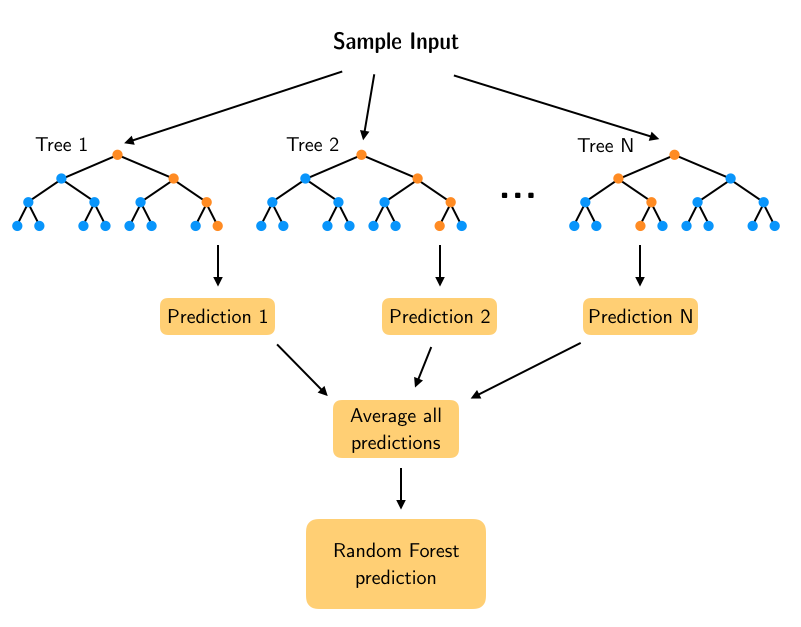
When we use a Random Forest to solve a regression task, the basic idea is that the leaf nodes of each Decision Tree predict a numerical value that is the average of the training instances associated with that node. These predictions are then averaged to obtain the final prediction from the forest of trees. In this lesson we will look at how we can build predictions from a single tree and get better predictions by adding progressively more trees to the forest.
# reload modules before executing user code
%load_ext autoreload
# reload all modules every time before executing Python code
%autoreload 2
# render plots in notebook
%matplotlib inline
# uncomment to update the library if working locally
# !pip install dslectures --upgrade
# data wrangling
import pandas as pd
import numpy as np
from numpy.testing import assert_array_equal
from dslectures.core import *
from dslectures.structured import *
from pathlib import Path
import pickle

# data viz
import matplotlib.pyplot as plt
import seaborn as sns
from sklearn.tree import plot_tree

sns.set(color_codes=True)
sns.set_palette(sns.color_palette("muted"))

# ml magic
from sklearn.model_selection import train_test_split
from sklearn.metrics import r2_score
from sklearn.ensemble import RandomForestRegressor
get_dataset('housing_processed.csv')
We also make use of the pathlib library to handle our filepaths:
DATA = Path('../data/')
!ls {DATA}
housing_data = pd.read_csv(DATA/'housing_processed.csv'); housing_data.head()
With the data loaded, we can recreate our feature matrix $X$ and target vector $y$ and train/validation splits as before.
As a sanity check, let's see how our baseline model performs on the validation set:
model = RandomForestRegressor(n_estimators=10, n_jobs=-1, random_state=42)
model.fit(X_train, y_train)
To simplify the evaluation of our models, let's write a simple function to keep track of the scores:
def print_rf_scores(fitted_model):
    """Generates RMSE and R^2 scores from fitted Random Forest model."""

    yhat_train = fitted_model.predict(X_train)
    R2_train = fitted_model.score(X_train, y_train)
    yhat_valid = fitted_model.predict(X_valid)
    R2_valid = fitted_model.score(X_valid, y_valid)

    scores = {
        "RMSE on train:": rmse(y_train, yhat_train),
        "R^2 on train:": R2_train,
        "RMSE on valid:": rmse(y_valid, yhat_valid),
        "R^2 on valid:": R2_valid,
    }
    if hasattr(fitted_model, "oob_score_"):
        scores["OOB R^2:"] = fitted_model.oob_score_

    for score_name, score_value in scores.items():
        print(score_name, round(score_value, 3))
print_rf_scores(model)
Let's build a model that is so simple that we can actually take a look at it. As we saw in lesson 4, a Random Forest is a simply forest of decision trees, so let's begin by looking at a single tree (called estimators in scikit-learn):
model = RandomForestRegressor(n_estimators=1, max_depth=3, bootstrap=False, n_jobs=-1, random_state=42)
model.fit(X_train, y_train)
In the above we have fixed the following hyperparameters:
n_estimators = 1: create a forest with one tree, i.e. a decision treemax_depth = 3: how deep or the number of "levels" in the treebootstrap=False: this setting ensures we use the whole dataset to build the tree
Let's see how this simple model performs:
print_rf_scores(model)
Unsurprisingly, this single tree yields worse predictions ($R^2 = 0.53$) than our baseline with 10 trees ($R^2 = 0.78$). Nevertheless, we can visualise the tree by accessing the estimators_ attribute and making use of scikit-learn's plotting API (link):
# get column names
feature_names = X_train.columns
# we need to specify the background color because of a bug in sklearn
fig, ax = plt.subplots(figsize=(30,10), facecolor='k')
# generate tree plot
plot_tree(model.estimators_[0], filled=True, feature_names=feature_names, ax=ax)
plt.show()

From the figure we observe that a tree consists of a sequence of binary decisions, where each box includes information about:
- The binary split criterion (mean squared error (mse) in this case)
- The number of
samplesin each node. Note we start with the full dataset in the root node and get successively smaller values at each split. - Darker colours indicate a higher
value, wherevaluerefers to the average of of the prices. - The best single binary split is for
median_income <= 4.068which improves the mean squared error from 9.3 billion to 6.0 billion.
Right now our simple tree model has $R^2 = 0.53$ on the validation set - let's make it better by removing the max_depth=3 restriction:
model = RandomForestRegressor(n_estimators=10, bootstrap=False, n_jobs=-1, random_state=42)
model.fit(X_train, y_train)
print_rf_scores(model)
Note that removing the max_depth constraint has yielded a perfect $R^2=1$ on the training set! That is because in this case each leaf node has exactly one element, so we can perfectly segment the data. We also have $R^2 = 0.64$ on the validation set which is better than our shallow tree, but we can do better.
Bagging is a technique that can be used to improve the ability of models to generalise to new data.
The basic idea between bagging is to consider training several models, each of which is only partially predictive, but crucially, uncorrelated. Since these models are effectively gaining different insights into the data, by averaging their predictions we can create an ensemble that is more predictive!
As shown in the figure, bagging is a two-step process:
- Bootstrapping, i.e. sampling the training set
- Aggregation, i.e. averaging predictions from multiple models
This gives us the acronym Bootstrap AGGregatING, or bagging for short 🤓.
The key for this to work is to ensure the errors of each mode are uncorrelated, so the way we do that with trees is to sample with replacement from the data: this produces a set of independent samples upon which we can train our models for the ensemble.
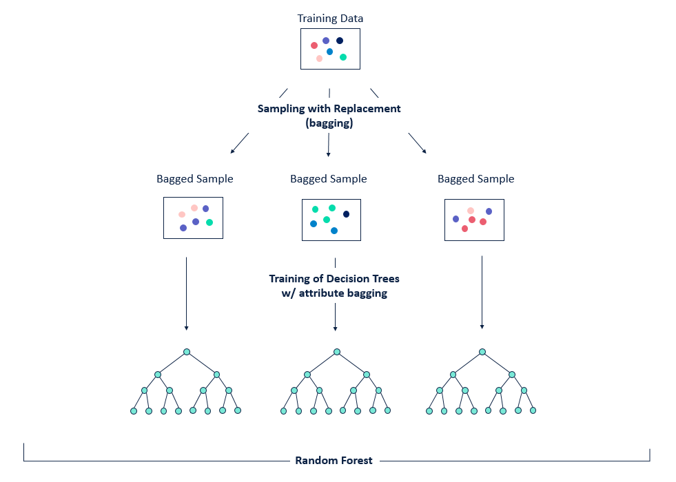
Figure reference: https://bit.ly/33tGPVT
If we revisit our very first model, we saw that the number of trees (n_estimators) is one of the parameters we can tune when building our Random Forest. Let's look at this more closely and see how the performance of the forest improves as we add trees.
model = RandomForestRegressor(n_estimators=10, bootstrap=True, n_jobs=-1, random_state=42)
model.fit(X_train, y_train)
After training, each tree is stored in an attribute called estimators_. For each tree, we can call predict() on the validation set and use the numpy.stack() function to concatenate the predictions together:
preds = np.stack([tree.predict(X_valid) for tree in model.estimators_])
Since we have 10 trees and 3889 samples in our validation set, we expect that preds will have shape $(n_\mathrm{trees}, n_\mathrm{samples})$:
preds.shape
Note: To calculate preds we made use of Python's list comprehension. An alternative way to do this would be to use a for-loop as follows:
preds_list = []

for tree in model.estimators_:
    preds_list.append(tree.predict(X_valid))

# concatenate list of predictions into single array
preds_v2 = np.stack(preds_list)

# test that arrays are equal
assert_array_equal(preds, preds_v2)
Let's now look at a plot of the $R^2$ values as we increase the number of trees.
def plot_r2_vs_trees(preds, y_valid):
    """Generate a plot of R^2 score on validation set vs number of trees in Random Forest"""
    fig, ax = plt.subplots()
    plt.plot(
        [
            r2_score(y_valid, np.mean(preds[: i + 1], axis=0))
            for i in range(len(preds) + 1)
        ]
    )
    ax.set_ylabel("$R^2$ on validation set")
    ax.set_xlabel("Number of trees")
plot_r2_vs_trees(preds, y_valid)

As we add more trees, $R^2$ improves but appears to flatten out. Let's test this numerically.
So far, we've been using a validation set to examine the effect of tuning hyperparameters like the number of trees - what happens if the dataset is small and it may not be feasible to create a validation set because you would not have enough data to build a good model? Random Forests have a nice feature called Out-Of-Bag (OOB) error which is designed for just this case!
The key idea is to observe that the first tree of our ensemble was trained on a bagged sample of the full dataset, so if we evaluate this model on the remaining samples we have effectively created a validation set per tree. To generate OOB predictions, we can then average all the trees and calculate RMSE, $R^2$, or whatever metric we are interested in.
To toggle this behaviour in scikit-learn, one makes use of the oob_score flag, which adds an oob_score_ attribute to our model that we can print out:
model = RandomForestRegressor(n_estimators=40, bootstrap=True, n_jobs=-1, oob_score=True, random_state=42)
model.fit(X_train, y_train)
print_rf_scores(model)
OOB score is handy when you want to find the best set of hyperparameters in some automated way. For example, scikit-learn has a function called grid search that allows you pass a list of hyperparameters and a range of values to scan through. Using the OOB score to evaluate which combination of parameters is best is a good strategy in practice.
Let's look at a few more hyperparameters that can be tuned in a Random Forest. From our earlier analysis, we saw that 40 trees gave good performance, so let's pick that as a baseline to compare against.
model = RandomForestRegressor(n_estimators=40, bootstrap=True, n_jobs=-1, oob_score=True, random_state=42)
model.fit(X_train, y_train)
print_rf_scores(model)
The hyperparameter min_samples_leaf controls whether or not the tree should continue splitting a given node based on the number of samples in that node. By default, min_samples_leaf = 1, so each tree will split all the way down to a single sample, but in practice it can be useful to work with values 3, 5, 10, 25 and see if the performance improves.
Another good hyperparameter to tune is max_features, which controls what random number or fraction of columns we consider when making a single split at a tree node. Here, the motivation is that we might have situations where a few columns in our data are highly predictive, so each tree will be biased towards picking the same splits and thus reduce the generalisation power of our ensemble. To counteract that, we can tune max_features, where good values to try are 1.0, 0.5, log2, or sqrt.