![]()
![]()
References
- Greedy function approximation: a gradient boosting machine by J. Friedman
# reload modules before executing user code
%load_ext autoreload
# reload all modules every time before executing Python code
%autoreload 2
# render plots in notebook
%matplotlib inline
# uncomment this if running locally or on Google Colab
# !pip install --upgrade hepml
# data wrangling
import pandas as pd
import numpy as np
from pathlib import Path
from fastprogress import progress_bar

# data viz
import matplotlib.pyplot as plt
import seaborn as sns
from hepml.core import plot_regression_tree, plot_predictions

sns.set(color_codes=True)
sns.set_palette(sns.color_palette("muted"))

# ml magic
from sklearn.ensemble import GradientBoostingRegressor, GradientBoostingClassifier
from sklearn.tree import DecisionTreeRegressor
from sklearn.model_selection import train_test_split, RandomizedSearchCV
from sklearn.metrics import mean_squared_error, roc_auc_score, accuracy_score
Plan of attack
Similar to how we implemented a Random Forest classifier from scratch in lesson 3, our strategy here will be to implement a Gradient Boosting regressor and compare against scikit-learn's version to make sure we are on the right track. The generalisation to classification tasks is left as an exercise for the intrepid student 🤓.
To guide our implementation, we will follow the least squares regression algorithm from Friedman's original paper on gradient boosting:
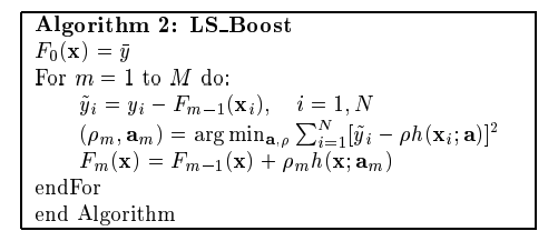
To keep things simple, we will test our implementation on the noisy quadratic dataset from lesson 4:
number_of_examples = 100
# fix the seed for reproducibility
np.random.seed(42)
# generate features
X = np.random.rand(number_of_examples, 1) - 0.5
# generate target
y = 3 * X[:, 0] ** 2 + 0.05 * np.random.randn(number_of_examples)
# create pandas.DataFrame
data = pd.DataFrame(data=np.stack([X[:, 0], y], axis=1), columns=["X", "y"])
data.head()
sns.scatterplot(x="X", y="y", data=data)
plt.show()

To get started, we need a data structure that will represent our boosted ensemble of regression trees. As a first guess, the variables we'll need to initialise our ensemble might include:
n_trees: how many trees or "stages" we sequentially add to the ensemblelearning_rate: a hyperparameter to control the contribution of each treemax_depth: a hyperparameter to control how deep each regression tree is (typically we want weak learners, i.e. shallow trees)
Unlike lesson 3, we will follow the fit-predict paradigm of scikit-learn and pass X and y in a dedicated fit function. With these considerations, let's go ahead and build our boosted ensemble class!
class LSBoost:
    def __init__(self, n_trees: int = 100, learning_rate: float = 0.1, max_depth: int = 3):
        self.n_trees = n_trees
        self.learning_rate = learning_rate
        self.max_depth = max_depth

        self.loss = LeastSquares()
        self.trees = [self.create_tree() for _ in range(self.n_trees)]

    def create_tree(self):
        return DecisionTreeRegressor(max_depth=self.max_depth)

    def fit(self, X, y):
        pass

    def predict(self, X):
        pass
Next let's try to instantiate our class:
lsb = LSBoost(n_trees=3)
Aha, we forgot to define our loss function! Following the analysis from Friedman's paper, for the LSBoost algorithm we need the Least Squares loss function
$$ L(y, F_M(X)) = \frac{1}{2}\sum_{i=1}^N \left(y_i - F_M(x_i) \right)^2 $$
which can be implemented in code as follows:
class LeastSquares:
    def __init__(self):
        pass

    def loss(self, y, y_pred):
        return 0.5 * (y - y_pred) ** 2

    def gradient(self, y, y_pred):
        return -(y - y_pred)
Now that the loss function is defined, we can now instantiate our ensemble class:
LSBoost.loss = LeastSquares()
lsb = LSBoost(n_trees=3)
lsb.trees
At the moment we just have an ensemble of tree regressors that have been initialised but not yet fit to data. To remedy that, recall that we first initialise a model with a constant value
$$ F_0(x) = \bar{y}$$
and then update this constant value by fitting regression trees to the gradient of the loss, also referred to as the pseudo-residuals:
$$ \tilde{y}_i = - \left[ \frac{\partial L(y_i, F(x_i)}{\partial F(x_i)} \right]_{F(x)=F_{m-1}(x)} = y_i - F_{m-1}(x_i) \,, \qquad i = 1, \ldots , N$$
Once the tree is fit to the gradients, we update the predictors as follows:
$$ F_{m+1}(X) = F_m(X) + \eta h_m(X)$$
where $\eta$ is the learning rate. We can implement these steps in code as follows:
def fit(self, X, y):
    # initial model - in this case the mean
    y_pred = np.full(np.shape(y), np.mean(y, axis=0))
    for i in progress_bar(range(self.n_trees)):
        gradient = self.loss.gradient(y, y_pred)
        # negative gradient equivalent to pseudo-residuals
        self.trees[i].fit(X, -gradient)
        # generate predictions from current tree
        update = self.trees[i].predict(X)
        # update prediction from composite model
        y_pred += self.learning_rate * update
Next let's override the base function of our class and fit to the training set:
LSBoost.fit = fit

lsb.fit(X, y)
Let's test whether this is working as expected by visualising a single tree in our ensemble:
plot_regression_tree(lsb.trees[0], data.columns, fontsize=22)

Comparison with scikit-learn's implementation yields a consistent result
gbr = GradientBoostingRegressor(n_estimators=3)
gbr.fit(X, y)

plot_regression_tree(gbr.estimators_[0][0], data.columns, fontsize=18)

and thus we can be confident that we've successfully implemented the first two steps of the LSBoost algorithm (namely adding a predictions of a single tree to the mean of $y$)!
The final step is to implement the functionality to generate predictions. As we saw in lesson 4, this is quite simple as we just need to add the predictions of each regression tree, weighted by the learning rate:
def predict(self, X):
    # initial prediction F_0
    initial_pred = np.full(np.shape(y), np.mean(y, axis=0))
    # composite tree predictions F_1 ... F_M
    tree_preds = sum(self.learning_rate * tree.predict(X) for tree in self.trees)
    return initial_pred + tree_preds
Let's override our base function and compare the error our model makes against the scikit-learn implementation:
LSBoost.predict = predict
def calculate_model_error(learning_rate, n_trees, max_depth):
    lsb = LSBoost(n_trees=n_trees, learning_rate=learning_rate, max_depth=max_depth)
    lsb.fit(X, y)
    lsb_preds = lsb.predict(X)

    gbr = GradientBoostingRegressor(n_estimators=n_trees)
    gbr.fit(X, y)
    gbr_preds = lsb.predict(X)

    print(f'MSE: {mean_squared_error(gbr_preds, lsb_preds):.16f}')
n_trees, max_depth, learning_rate = 100, 3, 0.5

calculate_model_error(learning_rate, n_trees, max_depth)

As a final sanity check, let's see if we can recover the boosting predictions from lesson 4:
n_trees, max_depth, learning_rate = 3, 2, 1.0

lsb = LSBoost(learning_rate=learning_rate, n_trees=n_trees, max_depth=max_depth)
lsb.fit(X, y)

gbr = GradientBoostingRegressor(learning_rate=learning_rate, n_estimators=n_trees, max_depth=max_depth)
gbr.fit(X, y)

fig, (ax0, ax1) = plt.subplots(ncols=2, figsize=(20,5))

plt.subplot(ax0)
plot_predictions(
    [lsb], X, y, axes=[-0.5, 0.5, -0.1, 0.8], label="LSBoost predictions", style="g-", data_label="Training set"
)

plt.subplot(ax1)
plot_predictions(
    [lsb], X, y, axes=[-0.5, 0.5, -0.1, 0.8], label="Scikit-learn predictions", style="g-", data_label="Training set"
)
plt.tight_layout()

Gradient boosting on the SUSY dataset
Now that we have understand how basic gradient boosting works, let's return to our SUSY dataset from previous lessons and apply gradient boosting to binary classification using scikit-learn's estimator and an experimental, but high-performance version based on histograms.
download_dataset("susy_sample.feather")
DATA = Path("../data")
!ls {DATA}
With pathlib it is a simple matter to define the filepath to the dataset, and since the file is in Feather format we can load it as a pandas.DataFrame as follows:
susy_sample = pd.read_feather(DATA / "susy_sample.feather")
susy_sample.head()
# sanity check on number of events
assert len(susy_sample) == 100_000
Next we create the feature matrix $X$ and target vector $y$, along with the training and validation sets:
X = susy_sample.drop("signal", axis=1)
y = susy_sample["signal"]

X_train, X_valid, y_train, y_valid = train_test_split(X, y, test_size=0.2, random_state=42)

print(f"Dataset split: {len(X_train)} train rows + {len(X_valid)} valid rows")
To get started lets create a baseline model using the default parameters of scikit-learn:
gbc = GradientBoostingClassifier(random_state=42)

%time gbc.fit(X_train, y_train)
We can score this model using our evaluation function from previous lessons:
def print_scores(fitted_model):
    res = {
        "Accuracy on train:": accuracy_score(fitted_model.predict(X_train), y_train),
        "ROC AUC on train:": roc_auc_score(
            y_train, fitted_model.predict_proba(X_train)[:, 1]
        ),
        "Accuracy on valid:": accuracy_score(fitted_model.predict(X_valid), y_valid),
        "ROC AUC on valid:": roc_auc_score(
            y_valid, fitted_model.predict_proba(X_valid)[:, 1]
        ),
    }
    if hasattr(fitted_model, "oob_score_"):
        res["OOB accuracy:"] = fitted_model.oob_score_

    for k, v in res.items():
        print(k, round(v, 3))
print_scores(gbc)
With a ROC AUC score of 0.87, our gradient boosted model is as good as the tuned Random Forest from lesson 2! Compared to the benchmark models in the SUSY article
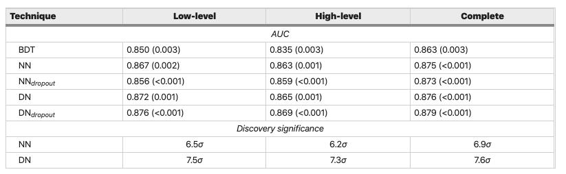
Figure reference: https://www.nature.com/articles/ncomms5308
we're also doing better than their Boosted Decision Tree (BDT) model and within 0.5-1% of the neural network based approaches. Let's see if we can make our model a bit better.
One major drawback with the GradientBoostingClassifier implementation is that it's extremely slow, partly because gradient boosting involves adding models sequentially and cannot be trivially parallelised like Random Forests. However, there are a few popular algorithms with provide significant performance speed-ups:
- XGBoost: for many years, this algorithm was the key ingredient behind Kaggle competitions.
- LightGBM: the new kid on the block, providing considerable performance gains over XGBoost.
Between them, these two algorithms represent the current state-of-the-art for training regression and classification models on tabular data (although see here for an example where deep learning yields the winning solution).
In this lesson, we will experiment with scikit-learn's historgram-based gradient boosting algorithm, which resembles LightGBM.
First we need to import the relevant class:
from sklearn.experimental import enable_hist_gradient_boosting
from sklearn.ensemble import HistGradientBoostingClassifier
hgb = HistGradientBoostingClassifier(random_state=42)

%time hgb.fit(X_train, y_train)
print_scores(hgb)
With a speedup of around 25x this isn't bad at all! We've also managed to boost our performance on the validation set using just the default parameters 🤓. We can also make things a little faster by employing early stopping in the same manner as lesson 4:
hgb = HistGradientBoostingClassifier(
    max_iter=100, validation_fraction=0.2, n_iter_no_change=5, tol=1e-5, random_state=42, warm_start=True
)
%time hgb.fit(X_train, y_train)
print(f"Optimal number of trees: {hgb.n_iter_}")
print(f"Minimum validation cross-entropy loss: {np.min(hgb.validation_score_)}")
In gradient boosting, the key hyperparameter to tune are the learning rate and number of "stages" or tree in the ensemble. Let's use randomised search to find a potential set of optimal values (we include max_depth for good measure):
# define range of values for each hyperparameter
param_dist = [
    {
        "learning_rate": [0.001, 0.01, 0.1, 0.2, 0.3, 0.5],
        "max_iter": [100, 250, 500, 1000],
        "max_depth": [2, 3, 5, 10]
    }
]

# instantiate baseline model
model = HistGradientBoostingClassifier()

# initialise random search with cross-validation
random_search = RandomizedSearchCV(
    model, param_distributions=param_dist, n_iter=40, cv=5, scoring="roc_auc", n_jobs=-1
)
# this is a RAM hungry monster, so best fed on a laptop!
%time random_search.fit(X, y)
Once the search is finished, we can get the best combination of parameters
random_search.best_params_
along with the best model:
best_model = random_search.best_estimator_
cv_results = random_search.cv_results_

for score, params in zip(cv_results["mean_test_score"], cv_results["params"]):
    print(f"{score:.3f}", params)
susy_test = pd.read_feather(DATA/'susy_test.feather')
X_test, y_test = susy_test.drop("signal", axis=1), susy_test["signal"]
# calculate probabilities per class
probs = best_model.predict_proba(X_test)[:, 1]

# evaluate against ground truth
roc_auc_score(y_test, probs)
- Implement gradient boosting from scratch for classification tasks. This is somewhat tricky - see here for the relevant ingredients.
- Pick one of the XGBoost or LightGBM libraries and see if you can use them to beat our ROC AUC score from the histogram-based classifier.