![]()
![]()
References
This lesson is based on the gradient boosting example from
- Chapter 7 of Hands-On Machine Learning with Scikit-Learn and TensorFlow by Aurèlien Geron
with parts of the theory coming from
- How to explain gradient boosting by Terence Parr and Jeremy Howard
- Gradient boosting explained by Ben Gorman
What is gradient boosting?
Boosting refers to an ensemble technique that combines multiple simple or "weak" models into a single composite model. Unlike the bagging method we saw in previous lessons, boosting methods train the models sequentially, where each model is chosen to improve the overall performance.
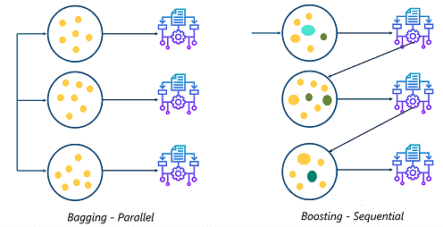
Figure reference: https://www.quora.com/Whats-the-difference-between-boosting-and-bagging
In gradient boosting, the trick is to fit each new model to the residual errors made by the previous one, e.g. the algorithm runs as follows:
- Fit a crappy model to the data $F_1(X) = y$
- Fit a crappy model to the residuals $h_1(X) = y - F_1(X)$
- Create a composite model $F_2(X) = F_1(X) + h_1(X)$
- Repeat steps 2 and 3 recursively $F_{m+1}(X) = F_m(X) + h_m(X)$ for $M$ steps until $F_M(X)$ is good enough. Note that our task at each step is to train the model $h_m(X) = y - F_m(X)$ on the residual errors.
For sufficiently large $M$, the result is a strong composite model $F_M(X) = \hat{y}$ that estimates the target values $y$.
$$ L(y, F_M(X)) = \frac{1}{N}\sum_{i=1}^N L(y_i, F_M(x_i)) $$
and for regression tasks it turns out that training models on the residual errors is equivalent to optimising the Mean Squared Error (MSE):
$$ L(y, F_M(X)) = \frac{1}{N}\sum_{i=1}^N \left(y_i - F_M(x_i) \right)^2 $$
In particular, for each $m\in 1, \ldots, M$ we calculate the gradient
$$ r_{im} = - \left[ \frac{\partial L(y_i, F(x_i)}{\partial F(x_i)} \right]_{F(x)=F_{m-1}(x)} \,, \qquad i = 1, \ldots , N$$
and fit a weak learner to these gradient components. The update step with gradient descent then looks like
$$ F_{m+1}(X) = F_m(X) + \gamma_m h_m(X)$$
where $\gamma_m$ is the learning rate or "shrinkage" parameter that controls the contribution of each tree (or how "far" a step we take in the direction of the average gradient).
In this lesson we look at the basic mechanics behind gradient boosting for regression tasks. The classification case is conceptually the same, but involves a different loss function and some technical details on how to combine predictions to build the ensemble.
# reload modules before executing user code
%load_ext autoreload
# reload all modules every time before executing Python code
%autoreload 2
# render plots in notebook
%matplotlib inline
# uncomment this if running locally or on Google Colab
# !pip install --upgrade hepml
# data wrangling
import pandas as pd
import numpy as np

# data viz
import matplotlib.pyplot as plt
import seaborn as sns
from hepml.core import plot_regression_tree

sns.set(color_codes=True)
sns.set_palette(sns.color_palette("muted"))

# ml magic
from sklearn.ensemble import GradientBoostingRegressor
from sklearn.tree import DecisionTreeRegressor
from sklearn.model_selection import train_test_split
from sklearn.metrics import mean_squared_error
number_of_examples = 100
# fix the seed for reproducibility
np.random.seed(42)
# generate features
X = np.random.rand(number_of_examples, 1) - 0.5
# generate target
y = 3 * X[:, 0] ** 2 + 0.05 * np.random.randn(number_of_examples)
# create pandas.DataFrame
data = pd.DataFrame(data=np.stack([X[:, 0], y], axis=1), columns=["X", "y"])
data.head()
Next, let's visualise our training set:
sns.scatterplot(x="X", y="y", data=data)
plt.show()

To create a boosted regression model, we start by creating a crappy model that predicts the initial approximation of $y$. As discussed above it is common to use shallow Decision Trees, so let's fix the max_depth to a small number:
tree_1 = DecisionTreeRegressor(max_depth=2)
tree_1.fit(X, y)
The resulting tree can be visualised with a helper function from our hepml library:
plot_regression_tree(tree_1, data.columns, fontsize=24)

Note that this tree looks similar to the classification trees we have analysed in previous lessons. The main difference is that instead of predicting a discrete class like "signal" or "background" in each leaf node, a regression tree predicts a continuous value. This value is simply the average target value of the training examples associated with a given node.
The CART algorithm is also similar to classification, except we now split the training set to minimise the Mean Squared Error (MSE) instead og Gini impurity:
$$J(k, t_k) = \frac{m_\mathrm{left}}{m}\mathrm{MSE}_\mathrm{left} + \frac{m_\mathrm{right}}{m}\mathrm{MSE}_\mathrm{right} $$
where
$$ \mathrm{MSE}_\mathrm{node} = \sum_{i\in \mathrm{node}} \left(\hat{y}_\mathrm{node} - y^{(i)}\right)^2 \qquad \mathrm{and} \qquad \hat{y}_\mathrm{node} = \frac{1}{m_\mathrm{node}} \sum_{i\in \mathrm{node}} y^{(i)} $$Next, let's add a new column of predictions to our pandas.DataFrame
data["Tree 1 prediction"] = tree_1.predict(X)
data.head()
and visualise the quality of the predictions on the training set:
def plot_predictions(regressors, X, y, axes, label=None, style="r-", data_style="b.", data_label=None):
    x1 = np.linspace(axes[0], axes[1], 500)
    y_pred = sum(regressor.predict(x1.reshape(-1, 1)) for regressor in regressors)
    plt.plot(X[:, 0], y, data_style, label=data_label)
    plt.plot(x1, y_pred, style, linewidth=2, label=label)
    if label or data_label:
        plt.legend(loc="upper center", fontsize=16)
    plt.axis(axes)
    plt.ylabel("$y$", fontsize=16)
    plt.xlabel("$X$", fontsize=16)
plot_predictions(
    [tree_1], X, y, axes=[-0.5, 0.5, -0.1, 0.8], label="$h(X)=h_1(X)$", style="g-", data_label="Training set"
)
plt.show()

Unsurprisingly, the weak model above is barely able to capture the structure of the data (i.e. it has high bias). However, we can improve the predictions by training a second regression tree on the residual errors made by the first tree:
data["Tree 1 residual"] = data["y"] - data["Tree 1 prediction"]
data.head()
tree_2 = DecisionTreeRegressor(max_depth=2)
tree_2.fit(X, data["Tree 1 residual"])
Now we have an ensemble consisting of two trees. We can get the predictions from the ensemble by simply summing the predictions across all trees:
data["Tree 2 prediction"] = tree_2.predict(X)
data["Tree 1 + tree 2 prediction"] = sum(tree.predict(X) for tree in (tree_1, tree_2))
data.head()
As before, we can plot the predictions of both our second tree on the residuals, along with the predictions from the ensemble on the training set:
fig, (ax0, ax1) = plt.subplots(ncols=2, figsize=(20, 5))

plt.subplot(ax0)
plot_predictions(
    [tree_2],
    X,
    data["Tree 1 residual"],
    axes=[-0.5, 0.5, -0.5, 0.5],
    label="$h_2(X)$",
    style="g-",
    data_style="k+",
    data_label="Residuals",
)
plt.ylabel("$y - h_1(X)$", fontsize=18)
plt.title("Residuals and tree predictions", fontsize=16)

plt.subplot(ax1)
plot_predictions([tree_1, tree_2], X, y, axes=[-0.5, 0.5, -0.1, 0.8], label="$h(X) = h_1(X) + h_2(X)$")
plt.title("Ensemble predictions", fontsize=16)
plt.tight_layout()

From the figure, we see that the ensemble's predictions have improved compared to our first crappy model!
It is not hard to see how we can continue this procedure by successively adding new models:
$$ F_{m+1}(x) = F_m(x) + h_m(x)\,, \qquad \mathrm{for} \, m \geq 0 $$
data["Tree 1 + tree 2 residual"] = data["Tree 1 residual"] - data["Tree 2 prediction"]
data.head()
tree_3 = DecisionTreeRegressor(max_depth=2)
tree_3.fit(X, data["Tree 1 + tree 2 residual"])
data["Tree 3 prediction"] = tree_3.predict(X)
data["Tree 1 + tree 2 + tree 3 prediction"] = sum(tree.predict(X) for tree in (tree_1, tree_2, tree_3))
data["Final residual"] = data["Tree 1 + tree 2 residual"] - data["Tree 3 prediction"]
data.head()
fig, (ax0, ax1) = plt.subplots(ncols=2, figsize=(20, 5))

plt.subplot(ax0)
plot_predictions(
    [tree_3],
    X,
    data["Tree 1 + tree 2 residual"],
    axes=[-0.5, 0.5, -0.5, 0.5],
    label="$h_3(X)$",
    style="g-",
    data_style="k+",
)
plt.ylabel("$y - h_1(X) - h_2(X)$", fontsize=16)

plt.subplot(ax1)
plot_predictions(
    [tree_1, tree_2, tree_3], X, y, axes=[-0.5, 0.5, -0.1, 0.8], label="$h(X) = h_1(X) + h_2(X) + h_3(X)$",
)
plt.tight_layout()

As promised, adding more models to the ensemble improves the predictions (at least qualitatively)!
Manually building up the gradient boosting ensemble is a drag, so in practice it is better to make use of scikit-learn's GradientBoostingRegressor class. Similar to the Random Forest classes that we've worked with in previous lessons, it has similar hyperparameters like max_depth and min_samples_leaf that control the growth of each tree, along with parameters like n_estimators which control the size of the ensemble. For example, we can reconstruct our hand-crafted ensemble from before as follows:
gbrt = GradientBoostingRegressor(max_depth=2, n_estimators=3, learning_rate=1.0)
gbrt.fit(X, y)
plot_predictions(
    [gbrt], X, y, axes=[-0.5, 0.5, -0.1, 0.8], label="Ensemble predictions", style="g-", data_label="Training set"
)
plt.show()

There are two main hyperparameters that you need to tune to prevent a boosted regression ensemble from overfitting the training set:
learning_rate: this hyperparameter weights the contribution of each tree. Low values like 0.1 imply more trees are needed in the ensemble, but will typically lead to better generalisation error.n_estimators: this hyperparameter controls the number of trees in the ensemble. Adding too many trees can lead to overfitting.
To show the effect of the learning rate, let's train two ensembles at different extremes:
gbrt_high_lr = GradientBoostingRegressor(max_depth=2, n_estimators=3, learning_rate=0.1, random_state=42)
gbrt_high_lr.fit(X, y)

gbrt_low_lr = GradientBoostingRegressor(max_depth=2, n_estimators=200, learning_rate=0.1, random_state=42)
gbrt_low_lr.fit(X, y)
fig, (ax0, ax1) = plt.subplots(ncols=2, figsize=(20, 5))

plt.subplot(ax0)
plot_predictions([gbrt_high_lr], X, y, axes=[-0.5, 0.5, -0.1, 0.8], label="Ensemble predictions")
plt.title(f"learning_rate={gbrt_high_lr.learning_rate}, n_estimators={gbrt_high_lr.n_estimators}", fontsize=18)

plt.subplot(ax1)
plot_predictions([gbrt_low_lr], X, y, axes=[-0.5, 0.5, -0.1, 0.8])
plt.title(f"learning_rate={gbrt_low_lr.learning_rate}, n_estimators={gbrt_low_lr.n_estimators}", fontsize=18)

plt.tight_layout()

In practice the learning rate and number of trees in the ensemble are found via cross-validation. However, it has been observed empircally that small learning rates like 0.1 produce models that generalise better. For fixed learing rate, we can find the optimal number of trees using a technique known as "early stoppping". Here the idea is to use a validation set to measure how the error decreases as we add more trees and find the optimal point from the curve:
X_train, X_valid, y_train, y_valid = train_test_split(X, y, random_state=49)

gbrt = GradientBoostingRegressor(max_depth=2, n_estimators=120, random_state=42)
gbrt.fit(X_train, y_train)

errors = [mean_squared_error(y_valid, y_pred) for y_pred in gbrt.staged_predict(X_valid)]
bst_n_estimators = np.argmin(errors) + 1

gbrt_best = GradientBoostingRegressor(max_depth=2, n_estimators=bst_n_estimators, random_state=42)
gbrt_best.fit(X_train, y_train)
min_error = np.min(errors)

fig, (ax0, ax1) = plt.subplots(ncols=2, figsize=(20, 5))

plt.subplot(ax0)
plt.plot(errors, "b.-")
plt.plot([bst_n_estimators, bst_n_estimators], [0, min_error], "k--")
plt.plot([0, 120], [min_error, min_error], "k--")
plt.plot(bst_n_estimators, min_error, "ko")
plt.text(bst_n_estimators, min_error * 1.2, "Minimum", ha="center", fontsize=14)
plt.axis([0, 120, 0, 0.01])
plt.xlabel("Number of trees", fontsize=16)
plt.ylabel("MSE", fontsize=16)
plt.title("Validation error", fontsize=14)

plt.subplot(ax1)
plot_predictions([gbrt_best], X, y, axes=[-0.5, 0.5, -0.1, 0.8])
plt.title(f"Best model ({bst_n_estimators} trees)", fontsize=14)

plt.tight_layout()

In practice it is better to actually stop the training when the early stopping criterion is met, instead of training many redundant models. In scikit-learn, this is configured by setting warm_start=True which allows for incremental training and can be use to stop the training loop when some threshold is met, e.g.
gbrt = GradientBoostingRegressor(
    n_estimators=120, validation_fraction=0.2, n_iter_no_change=5, tol=1e-5, max_depth=2, random_state=42, warm_start=True
)
gbrt.fit(X, y)
print(f"Optimal number of trees: {gbrt.n_estimators_}")
print(f"Minimum validation MSE: {np.min(gbrt.train_score_)}")

plot_predictions([gbrt], X, y, axes=[-0.5, 0.5, -0.1, 0.8])

Use scikit-learn's GradientBoostingClassifier to explore how the algorithm's hyperparameters influence the decision boundary on the following synthetic dataset for binary classification:
from sklearn.datasets import make_moons

X, y = make_moons(n_samples=500, noise=0.30, random_state=42)

sns.scatterplot(x=X[:, 0], y=X[:, 1], hue=y)
plt.xlabel("$x_1$")
plt.ylabel("$x_2$")
plt.show()

In addition, see if you can use early stopping to find the optimal number of trees to include in the ensemble.