Lecture 4 - Jet images and transfer learning with CNNs#

A look at converting jets into images and classifying them with convolutional neural networks

Learning objectives#

Understand how to convert jets into images
Know what transfer learning is and it’s advantages compared to training a neural network from scratch
Understand the main steps needed to fine-tune a convolutional neural network

References#

Chapter 1 of Deep Learning for Coders with fastai & PyTorch by Jeremy Howard and Sylvain Gugger.
The Machine Learning Landscape of Top Taggers by G. Kasieczka et al.
Jet-Images – Deep Learning Edition by L. de Oliviera et al.

Setup#

# Uncomment and run this cell if using Colab, Kaggle etc
# %pip install fastai==2.6.0 datasets energyflow huggingface_hub

Imports#

import pandas as pd
from datasets import load_dataset
from energyflow.utils import (
    center_ptyphims,
    phi_fix,
    pixelate,
    ptyphims_from_p4s,
    reflect_ptyphims,
    rotate_ptyphims,
)
from fastai.vision.all import *
from huggingface_hub import from_pretrained_fastai
from sklearn.metrics import accuracy_score, auc, roc_auc_score, roc_curve
from torch.utils.data import Dataset, TensorDataset
from torchvision.transforms import ToTensor
from scipy.interpolate import interp1d

import datasets

# Suppress logs to keep things tidy
datasets.logging.set_verbosity_error()

Creating jet images#

As we saw in lectures 1 and 2, there are various ways to represent jet data for neural networks. So far, we’ve focused on \(N\)-subjettiness features \(\tau_N^{\beta}\), which represent jets in a tabular format. Today, we’ll examine another popular representation that treats jets as 2D images. An example from the top tagging review is shown below:

But why consider images in the first place? The motivation here is partly historical: computer vision is where the deep learning revolution started in 2011, with DanNet and AlexNet smashing the state-of-the-art on popular benchmarks. Both approaches were based on a type of architecture called a convolutional neural network (CNN), which is especially well suited for analysing images. In the next lecture we’ll examine how CNNs work in detail, so today we’ll focus on creating jet images and training a CNN with the high-level API of fastai.

To get started, let’s take a look at how we can construct images from the 4-vectors associated with the consituents in a jet. We’ll use the raw events from the Top Quark Tagging dataset in lecture 1, so let’s download it and grab a sample of 10,000 events to play with:

raw_events = load_dataset("dl4phys/top_tagging", split="validation")
sample_df = raw_events.shuffle(seed=42).select(range(10_000)).to_pandas()
sample_df.head()

	E_0	PX_0	PY_0	PZ_0	E_1	PX_1	PY_1	PZ_1	E_2	PX_2	...	truthE	truthPX	truthPY	truthPZ	ttv	is_signal_new
0	130.172562	114.353065	-59.476486	18.188450	58.261734	56.383465	-6.442986	-13.184177	43.596382	37.914547	...	496.599976	418.331940	-202.994308	43.685955	2	1
1	144.244232	44.394894	71.800972	-116.962021	176.547729	61.791088	51.010948	-157.317657	134.554794	47.264194	...	1061.465576	240.111099	465.869263	-906.836731	2	1
2	164.264938	29.799849	-155.011093	45.458752	154.540726	34.444710	-140.643768	53.997475	102.357109	19.766624	...	0.000000	0.000000	0.000000	0.000000	2	0
3	190.001175	-59.107372	-180.212479	11.411892	36.530270	-16.578011	-32.546757	0.582238	28.827248	-10.152600	...	0.000000	0.000000	0.000000	0.000000	2	0
4	197.350937	-190.924622	-28.691614	-40.889717	65.894730	-63.749012	-9.580021	-13.652922	53.116070	-52.294987	...	0.000000	0.000000	0.000000	0.000000	2	0

5 rows × 806 columns

Here we’ve used the shuffle() and select() methods to create a random sample, and then converted the result to a pandas DataFrame. It’s convenient to reshape the events so that instead of having 800 columns, we have 200 columns, where each column groups the 4-vectors of a constituent in a single array. We can do this by casting our DataFrame to NumPy and applying the reshape() method as follows:

# Reshape to size (num_jets, num_consituents, 4)
events = sample_df.iloc[:, :800].values.reshape(-1, 200, 4)
# Extract array of labels
labels = sample_df["is_signal_new"].values

events.shape, labels.shape

((10000, 200, 4), (10000,))

Now, each row in our events array corresponds to an array of shape (num_constituents, 4). We can inspect one of these constituent 4-vectors as follows:

events[0][0]

array([130.17256 , 114.353065, -59.476486,  18.18845 ], dtype=float32)

Rotating to hadronic coordinates#

Each of the 4-vectors in events is currently stored in Cartesian coordinates \((E, p_x, p_y, p_z)\). However, it is convenient to rotate the basis to hadronic coordinates \((p_T, y, \phi, m)\), where:

\[ p_T = \sqrt{p_x^2 + p_y^2} \,, \quad y = \mathrm{arctanh}\, \frac{p_z}{E} \,, \quad \phi = \arctan \frac{p_y}{p_x}\,, \quad m = \sqrt{E - p_x^2 - p_y^2 - p_z^2}\]

Here \(p_T\) denotes the transverse momentum, \(y\) is the rapidity, \(\phi\) the azimuthal angle, and \(m\) the mass. Although we could implement these formulas directly in NumPy, we’ll use the EnergyFlow library instead, which provides many utility functions for precisely these cases. To convert our 4-vectors to hadronic coordinates, we use the ptyphims_from_p4s() function:

events_hadronic = ptyphims_from_p4s(events, phi_ref="hardest", mass=True)

Here, the phi_ref argument specifies which \(\phi\) value to use as reference within \(\pm \pi\). The next step is to centre the collection of 4-vectors associated with each event. We can use the center_ptyphims() function to handle that for us:

events_centered = [center_ptyphims(event) for event in events_hadronic]

The final step is to reflect and rotate our events:

events_reflected_and_rotated = [
    reflect_ptyphims(rotate_ptyphims(event)) for event in events_centered
]

The final step is to create a jet image from an array of 4-vectors. Here we can use the pixelate() function from EnergyFlow and we’ll follow the precription from the top tagging review to create images of \(40\times 40\) pixels. The end result is as follows:

images = [
    pixelate(
        event,
        npix=40,
        img_width=0.8,
        nb_chan=1,
        norm=False,
        charged_counts_only=False,
    )
    for event in events_reflected_and_rotated
]

images = np.array(images).reshape(len(images), 40, 40)

Now that we have our images, let’s split them into those corresponding to the top-quarks and QCD background:

top_images = images[labels == 1]
qcd_images = images[labels == 0]

And now we can plot a few examples to see how the images look like:

for i in range(2):
    plt.figure(figsize=(8, 4))
    plt.subplot(1, 2, 1)
    plt.title("QCD background")
    plt.imshow(qcd_images[i])
    plt.subplot(1, 2, 2)
    plt.title("Top quark")
    plt.imshow(top_images[i])
    plt.tight_layout()
    plt.show()

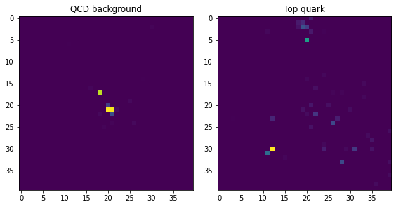
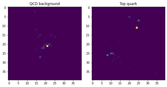
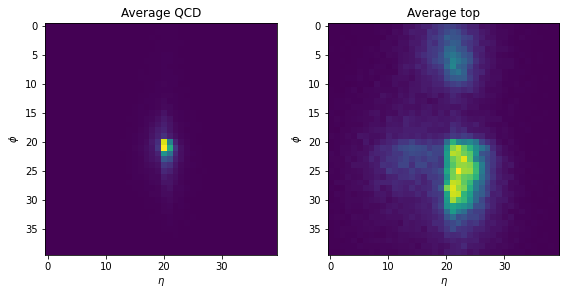
Notice how the background events are much more clustered around the centre, while the top-quark jets have multiple “prongs”. We can see this more clearly by averaging the pixel values across all events:

plt.figure(figsize=(8, 4))
plt.subplot(1, 2, 1)
plt.imshow(np.sum(qcd_images, axis=0))
plt.title("Average QCD")
plt.xlabel("$\eta$")
plt.ylabel("$\phi$")

plt.subplot(1, 2, 2)
plt.imshow(np.sum(top_images, axis=0))
plt.title("Average top")
plt.xlabel("$\eta$")
plt.ylabel("$\phi$")

plt.tight_layout()
plt.show()

Great, we now have a way to convert raw 4-vectors into jet images! For convenience, we’ve applied the above steps to the whole top_tagging dataset, so let’s download it now from the Hugging Face Hub:

images_ds = load_dataset("dl4phys/top_tagging_images")
images_ds

DatasetDict({
    validation: Dataset({
        features: ['image', 'label'],
        num_rows: 403000
    })
    test: Dataset({
        features: ['image', 'label'],
        num_rows: 404000
    })
    train: Dataset({
        features: ['image', 'label'],
        num_rows: 1211000
    })
})

Here we now have three splits to work with, and we can access an individual image by indexing as follows:

img = images_ds["train"][0]["image"]
plt.imshow(img);

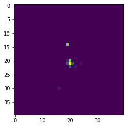
Okay, this looks like a jet image - let’s now take a look at converting them to PyTorch tensors that are suitable for training a neural net!

From images to tensors#

Now that we have a dataset of images, the next thing we need to do is convert them to PyTorch tensors and wrap them in a DataLoader. One way to do this is via torchvision’s ToTensor class, which converts a PIL image into a tensor as follows:

t = ToTensor()(img)
t.shape

torch.Size([1, 40, 40])

Here we can see that we now have a tensor of shape (num_channels, height, width), where num_channels is 1 because we’re dealing with black and white images, and height and width denote the number of pixels. To apply ToTensor to multiple images, we can use a list comprehension and torch.cat() to concatenate all the tensors as a single tensor:

x = torch.cat([ToTensor()(img) for img in images_ds["train"][:10]["image"]])
x.shape

torch.Size([10, 40, 40])

Now this isn’t quite what we want because CNNs in PyTorch expect rank-4 tensors with a shape (minibatch, channels, height, width), where channels refers to the number of color channels (e.g. RGB) of the image. In our case, the images are black and white, so we just need to reshape the tensor to insert a new dimension in the second position:

x = torch.cat([ToTensor()(img) for img in images_ds["train"][:10]["image"]])
x.unsqueeze_(dim=1)
x.shape

torch.Size([10, 1, 40, 40])

Great, we now have the image tensors in the right shape, so let write a simple get_dataset() helper function that applies this over a single training split:

def get_dataset(dataset, num_examples=None):
    if num_examples is not None:
        dataset = dataset.shuffle(seed=42).select(range(num_examples))

    x = torch.cat([ToTensor()(img) for img in dataset["image"]]).unsqueeze(1)
    y = torch.cat([torch.tensor(l).unsqueeze(0) for l in dataset["label"]])

    return TensorDataset(x, y)

Here we’ve also collected the labels in a single tensor and returned a TensorDataset object that we can iterate over:

# Lower the training size if Colab RAM explodes 💣
train_ds = get_dataset(images_ds["train"], num_examples=350_000)
valid_ds = get_dataset(images_ds["validation"], num_examples=50_000)

Now that we have the PyTorch datasets prepared, let’s wrap them in dataloaders so we can generate minibatches during training:

train_dl = DataLoader(train_ds, bs=128, shuffle=True)
valid_dl = DataLoader(valid_ds, bs=128)
dls = DataLoaders(train_dl, valid_dl)

Fine-tuning a pretrained CNN#

Now that we have prepared our data and created dataloaders, we can train a CNN! Instead of training a CNN from scratch, we’ll use a pretrained model that has been already been trained to classify over a million photos in the famous ImageNet dataset. These models are called “pretrained” because their weights have already been optimized by training on another dataset. The layers in a pretrained model are well suited for detecting edges, colour gradient and so on, which allows us to train a new model with much less labelled data, and much faster.

In practice, we replace the last layer of the pretrained model with a randomly initialized one that has the appropriate shape for the task at hand. For instance, ImageNet involves 1,000 different classes, so if we want to re-use the weights of a model trained on this dataset for a new set of classes, we’ll need to resize the last layer. This last layer is often referred to as the head of the network, with every layer before it belonging to the body.

This process of reusing the weights to solve a different task is called transfer learning, and now underpins much of the success that deep learning has achieved in computer vision, natural language processing, and audio. A cartoon of the process is shown below:

Anyway, enough jargon - let’s train a model! As we did in lecture 1, we’ll use the high-level API of fastai, which provides factory methods for various domains. Instead of a tabular_learner() we’ll use the vision_learner(), which is designed for computer vision tasks:

learn = vision_learner(
    dls,
    resnet34,
    metrics=[accuracy, RocAucBinary()],
    n_in=1,
    n_out=2,
    normalize=False,
    loss_func=F.cross_entropy,
)

Here we’ve provided the dataloaders and specified resnet34 as the name of the pretrained model we wish to initialise with. ResNets are a popular type of CNN that we might cover in a future lesson, but for now it is enough to know that they are great for most computer vision tasks. Now, because we’re using custom dataloaders instead of the factory methods provided by fastai, we need to specify that our model should run on a GPU instead of CPU (the default). We can do that by tapping into the model and selecting the desired device name with PyTorch’s to() method:

learn.model.to("cuda");

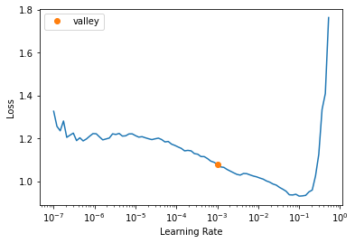
Now that our model is on the GPU, we can follow the same steps we’ve done in previous lectures. First we find a good learning rate:

learn.lr_find()

SuggestedLRs(valley=0.0010000000474974513)

And finally we can train the model:

learn.fine_tune(3, 3e-3)

Note that this time we didn’t call fit() or fit_one_cycle() as we’ve done in previous lectures. That’s because we’re starting with a pretrained model whose weights we “fine-tuned” to the new dataset of jet images. This process involves some tricks which is why it is called fine_tune(). Anyway, we’ve now got a model that scores pretty well on the validation set. Let’s compute the same metrics we did in lecture 1, but now on the test set:

def compute_metrics(learn, test_ds):
    test_dl = learn.dls.test_dl(test_items=test_ds)
    preds, targs = learn.get_preds(dl=test_dl)
    fpr, tpr, _ = roc_curve(y_true=targs, y_score=preds[:, 1])
    acc_test = accuracy_score(targs, preds.argmax(dim=-1))
    auc_test = auc(fpr, tpr)
    background_eff = interp1d(tpr, fpr)
    background_eff_at_30 = background_eff(0.3)

    print(f"Accuracy: {acc_test:.4f}")
    print(f"AUC: {auc_test:.4f}")
    print(
        f"Backround rejection at signal efficiency 0.3: {1/background_eff_at_30:0.3f}"
    )
    return fpr, tpr

test_ds = get_dataset(images_ds["test"])
_, _ = compute_metrics(learn, test_ds)

Comparing our results against those in the top tagging review, shows that our CNN is getting quite competitive results with the state-of-the-art!

Deep Learning for Particle Physicists

Lecture 4 - Jet images and transfer learning with CNNs

Contents