Lecture 2 - Gradient descent#

A look at optimising functions with gradient descent

Learning objectives#

Understand what stochastic gradient descent is and how to minimise functions with it in PyTorch

References#

This notebook is a condensed version of Chapter 4 of Deep Learning for Coders with fastai & PyTorch by Jeremy Howard and Sylvain Gugger. We recommend reading that chapter in detail to get the full context.

Setup#

# Uncomment and run this cell if using Colab, Kaggle etc
# %pip install fastai==2.6.0

Imports#

import torch
from fastai.tabular.all import *
from tqdm.auto import tqdm

Stochastic gradient descent#

What does it actually mean to train a model? In deep learning, this process is called stochastic gradient descent (SGD). As described in the fastai book, this process involves 7 main steps:

Initialize the parameters of the neural network
For each example in the dataset, use the parameters to make a predicition (e.g. is this jet produced by a top-quark or QCD background?)
Use these predictions to calculate the model performance via the loss
Calculate the gradients
Update all the parameters by taking a step in the direction that minimises the loss
Repeat from step 2
Stop the training process once the model is good enough

In this lecture, we will take a deep dive into how these steps work in PyTorch. But before doing that, let’s take a quick look at how gradients are computed in PyTorch, as they’ll play a large role in what follows.

Calculating gradients#

To illustrate how gradients are computed in PyTorch, let’s consider a simple quadratic loss function:

def f(x):
    return x**2

Next, let’s create a tensor at the point we wish to calculate the gradient of \(f(x)\):

xt = torch.tensor(3.0, requires_grad=True)
xt

tensor(3., requires_grad=True)

Here, the requires_grad argument tells PyTorch to begin recording operations on the tensor xt; in particular which parts of the code should be included for computing gradients. Next, let’s use this tensor to generate the output yt from our function:

yt = f(xt)
yt

tensor(9., grad_fn=<PowBackward0>)

This looks good and here PyTorch is indicating both the value of the tensor and the gradient function that will be used. So let’s now compute the gradients with the backward() method:

yt.backward()

Here, “backward” refers to backpropagation, which is the technique used in deep learning to compute the gradients of the loss with respect to all the parameters in the model. In this simple example we just have one parameter to consider, but in general, a neural network can have thousands to billions of parameters, and so an efficient method is needed to compute this many gradients efficiently.

Under the hood, PyTorch implements backprogations via an automatic differentiation engine called autograd that keeps a record of tensors and all executed operations (like sum, multiplication etc) as a directed acyclic graph (DAG). We’ll look at backpropagation in a bit more detail later, but for now the main thing to note is that the gradients are stored in the Tensor.grad attribute:

xt.grad

tensor(6.)

Great, this worked since we know analytically that \(f'(3) = 6\)! Now let’s generalise to the case where our tensor is an array of values:

xt = torch.tensor([3.0, 4.0, 10.0], requires_grad=True)
xt

tensor([ 3.,  4., 10.], requires_grad=True)

To compute the gradients, we’ll also need to add a sum() operator to our function so that it returns a scalar:

def f(x):
    return (x**2).sum()


yt = f(xt)
yt

tensor(125., grad_fn=<SumBackward0>)

Here we can see that passing an array of values and applying the sum is equivalent to computing:

\[ f(x_0) = \sum_i x_i^2 \Big|_{x_0} \]

Finally, let’s check the values of our gradients \(f'(x_0)\):

yt.backward()
xt.grad

tensor([ 6.,  8., 20.])

Now that we know how to compute gradients, we next need to find a way to update all the weights. Let’s take a look at this with a more realistic example.

A toy example#

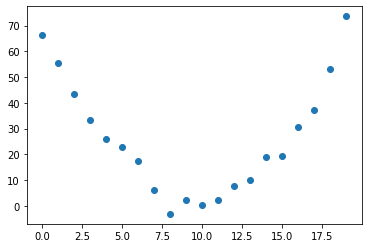
Imagine that you’re measuring some signal at fixed time steps:

time = torch.arange(0, 20).float()

and then find the result of your measurements looks something like a parabola:

signal = torch.randn(20) * 3 + 0.75 * (time - 9.5) ** 2 + 1  # 1 * (time - 10) ** 2 + 1
plt.scatter(time, signal);

Using SGD, our goal will be to find a function that best fits the data. A good choice of function would be a general quadratic of the form:

\[ f(t, a,b,c) = at^2 + bt + c \]

We can then define a function that collects the timestep \(t\) and the parameters \(a,b,c\) as separate arguments:

def f(t, params):
    a, b, c = params
    return a * (t**2) + (b * t) + c

To define what we mean by “best” values of \(a,b,c\), we’ll need to choose a loss function. For regression problems like ours, it is common to use the mean squared error, which we can define as follows:

def mse(preds, targets):
    return ((preds - targets) ** 2).mean()

Now that we have a function we with to optimise and a loss function, let’s work through the 7 steps of training a model.

Step 1: Initialize the parameters#

Since our function involves three parameters \(a,b,c\), we’ll initialise random values of them using the torch.randn() function:

set_seed(666)
params = torch.randn(3).requires_grad_()
params

tensor([-2.1188,  0.0635, -1.4555], requires_grad=True)

As we did earlier, we’ve applied the requires_grad_() method to indicate that we wish to track the gradients of the params tensor. We’ve also set the seed to the number of the beast so that the results are reproducible when you run the code on your own machine 😈.

Step 2: Calculate the predictions#

The next step is compute the predictions from the “model”:

preds = f(time, params)
preds.shape

torch.Size([20])

Notice that we get one prediction for each of the time step in the time array. We can visualise these predictions with the following helper function:

def show_preds(preds, ax=None):
    if ax is None:
        ax = plt.subplots()[1]
    ax.scatter(time, signal)
    ax.scatter(time, to_np(preds), color="red")
    plt.show()

show_preds(preds)

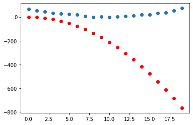
Unsuprisngly, our randomly initialised model isn’t very good - let’s see if we can improve it by adjusting the parameters!

Step 3: Calculate the loss#

To know how we should adjust the parameters, we need a way to indicate in which direction we should optimise them. To do so, we’ll first compute the loss:

loss = mse(preds, signal)
loss

tensor(143901.3594, grad_fn=<MeanBackward0>)

To improve this value (i.e. make it lower), we’ll need the gradients.

Step 4: Calculate the gradients#

Next we calculate the gradients:

loss.backward()
params.grad

tensor([-126948.2656,   -8149.7505,    -577.4262])

Step 5: Step the weights#

Next we need to update the parameters according to a learning rate. For now we’ll just ues \(10^{-5}\):

lr = 1e-5
params.data -= lr * params.data
params.grad = None

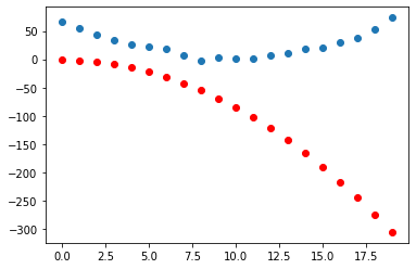
Let’s check if the loss has improved:

preds = f(time, params)
mse(preds, signal)

tensor(143898.6562, grad_fn=<MeanBackward0>)

show_preds(preds)

Okay, not much of a change after one step so let’s repeat the process a few times to see how things improve. To do so, we’ll create another helper function that combines all of the above logic:

def apply_step(params, prn=True):
    preds = f(time, params)
    loss = mse(preds, signal)
    loss.backward()
    params.data -= lr * params.grad.data
    params.grad = None
    if prn:
        print(f"Loss: {loss.item()}")
    return preds

Step 6: Repeat the process#

Now that we’ve done one step of gradient descent, it’s time to repeat a few times to see if the loss decreases:

num_of_iterations = 1_000_000

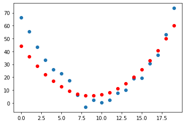
for iteration in tqdm(range(num_of_iterations)):
    if iteration % 200_000 == 0:
        print(f"Iteration: {iteration}")
        apply_step(params, prn=True)
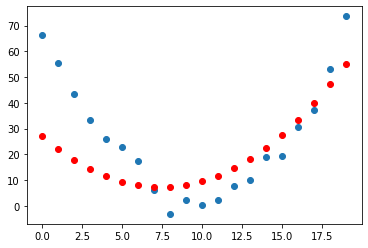
        preds = f(time, params)
        show_preds(preds)
    else:
        apply_step(params, prn=False)

Iteration: 0
Loss: 143898.65625

Iteration: 200000
Loss: 252.34817504882812

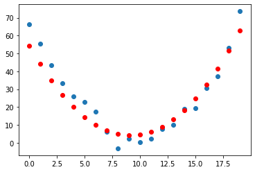
Iteration: 400000
Loss: 97.08727264404297

Iteration: 600000
Loss: 41.89081573486328

Iteration: 800000
Loss: 22.2598876953125

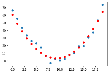
Great, this seems to work! The loss is decreasing with each step, indicating that a different quadratic function is being tried with different values of the parameters \(a,b,c\).

Step 7: Stop#

Here we stopped the process arbitrarily after 1 million steps, but in practice one would track metrics like accuracy and loss on a validation set to decide when is a good point to terminate the training.

All of these steps can be carried over to any deep learning problem, so next lecture we’ll see how all these steps can be applied to the jet tagging datasets from lecture 1!

Exercises#

Generate some random linear data and use SGD to find the best parameters for a linear regression model \(\hat{y} = h_\theta(\bf{x}) = \bf{\theta}\cdot {\bf x} + \theta_0 \)

Deep Learning for Particle Physicists

Lecture 2 - Gradient descent

Contents